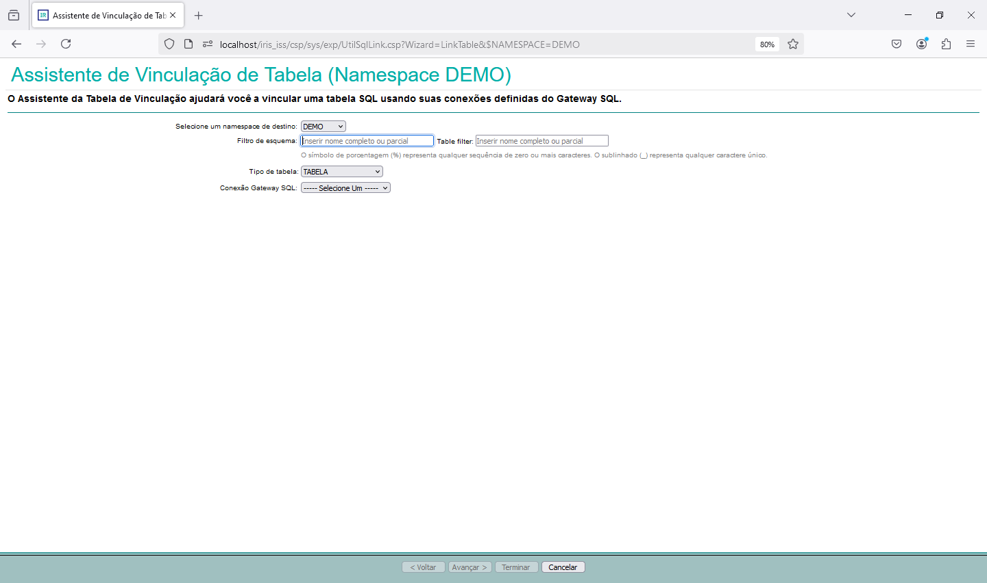
Using SQL Gateway with Python, Vector Search, and Interoperability in InterSystems Iris

Part 2 – Python and Vector Search

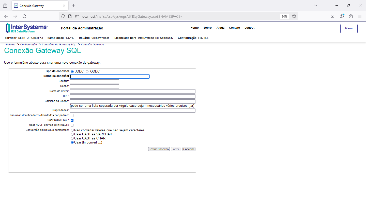
Since we have access to the data from our external table, we can use everything that Iris has to offer with this data. Let's, for example, read the data from our external table and generate a polynomial regression with it.

For more information on using python with Iris, see the documentation available at https://docs.intersystems.com/irislatest/csp/docbook/DocBook.UI.Page.cls?KEY=AFL_epython

Let's now consume the data from the external database to calculate a polynomial regression. To do this, we will use a python code to run a SQL that will read our MySQL table and turn it into a pandas dataframe:

ClassMethod CalcularRegressaoPolinomialODBC() As %String [ Language = python ]
{
    import iris
    import json
    import pandas as pd
    from sklearn.preprocessing import PolynomialFeatures
    from sklearn.linear_model import LinearRegression
    from sklearn.metrics import mean_absolute_error
    import numpy as np
    import matplotlib
    import matplotlib.pyplot as plt
    matplotlib.use("Agg")

    # Define Grau 2 para a regressão
    grau = 2
    
    # Recupera dados da tabela remota via ODBC
    rs = iris.sql.exec("select venda as x, temperatura as y from estat.fabrica")
    df = rs.dataframe()
   
    # Reformatando x para uma matriz 2D exigida pelo scikit-learn
    X = df[['x']]
    y = df['y']
    
    # Transformação para incluir termos polinomiais
    poly = PolynomialFeatures(degree=grau)
    X_poly = poly.fit_transform(X)

    # Inicializa e ajusta o modelo de regressão polinomial
    model = LinearRegression()
    model.fit(X_poly, y)

    # Extrai os coeficientes do modelo ajustado
    coeficientes = model.coef_.tolist()  # Coeficientes polinomiais
    intercepto = model.intercept_       # Intercepto
    r_quadrado = model.score(X_poly, y) # R Quadrado

    # Previsão para a curva de regressão
    x_pred = np.linspace(df['x'].min(), df['x'].max(), 100).reshape(-1, 1) 
    x_pred_poly = poly.transform(x_pred)
    y_pred = model.predict(x_pred_poly)
    
    # Calcula Y_pred baseado no X
    Y_pred = model.predict(X_poly)
            
    # Calcula MAE
    MAE = mean_absolute_error(y, Y_pred)
    
    # Geração do gráfico da Regressão
    plt.figure(figsize=(8, 6))
    plt.scatter(df['x'], df['y'], color='blue', label='Dados Originais')
    plt.plot(df['x'], df['y'], color='black', label='Linha dos Dados Originais')
    plt.scatter(df['x'], Y_pred, color='green', label='Dados Previstos')
    plt.plot(x_pred, y_pred, color='red', label='Curva da Regressão Polinomial')
    plt.title(f'Regressão Polinomial (Grau {grau})')
    plt.xlabel('X')
    plt.ylabel('Y')
    plt.legend()
    plt.grid(True)

    # Salvando o gráfico como imagem
    caminho_arquivo = 'c:\\temp\\RegressaoPolinomialODBC.png'
    plt.savefig(caminho_arquivo, dpi=300, bbox_inches='tight')
    plt.close()
    
    resultado = {
        'coeficientes': coeficientes,
        'intercepto': intercepto,
        'r_quadrado': r_quadrado,
        'MAE': MAE
    }

    return json.dumps(resultado)
}

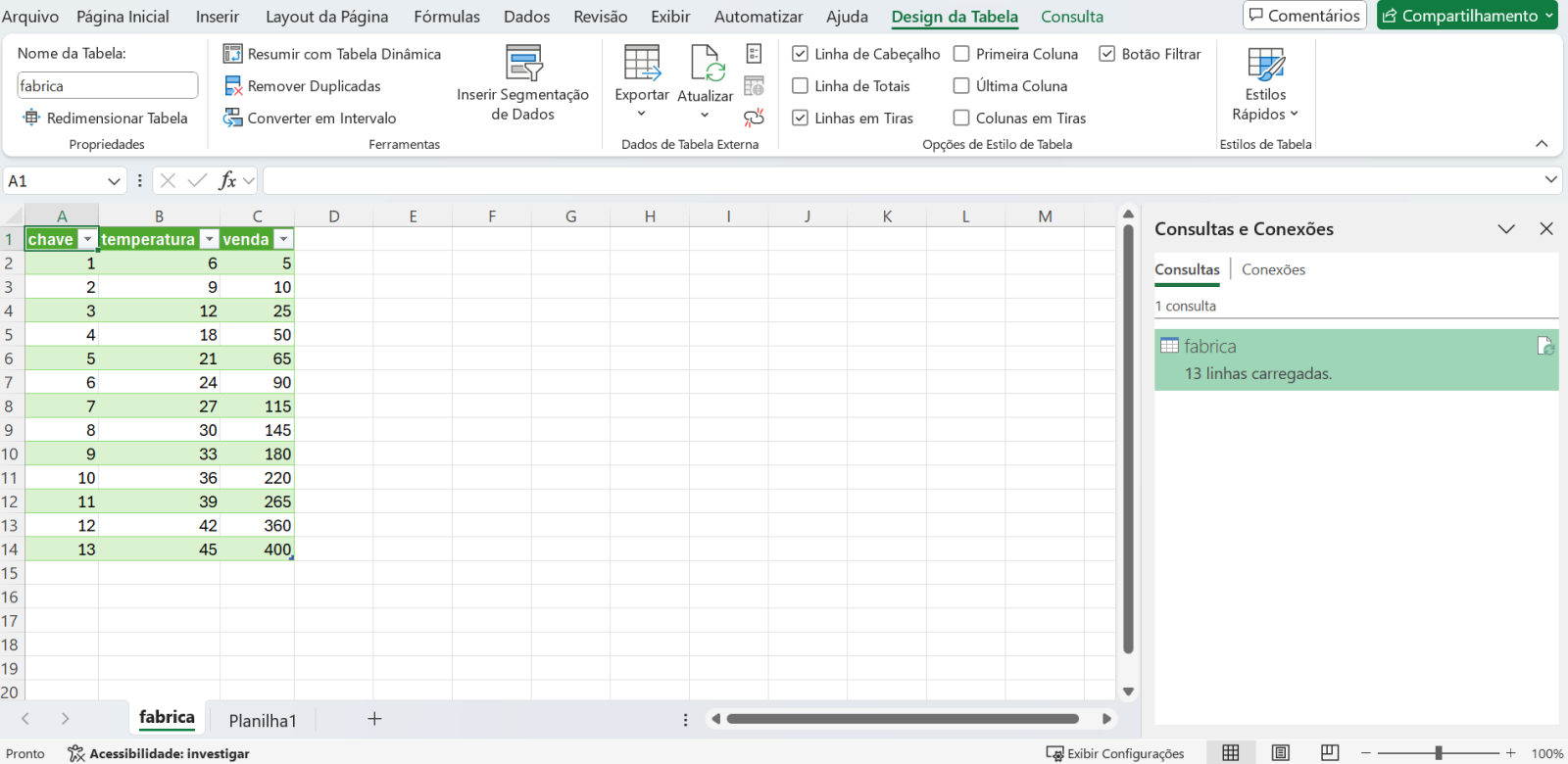
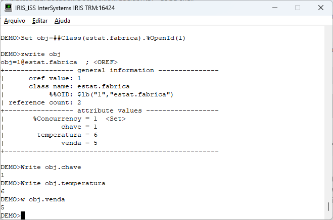
The first action we take in the code is to read the data from our external table via SQL and then turn it into a Pandas dataframe. Always remembering that the data is physically stored in MySQL and is accessed via ODBC through the SQL Gateway configured in Iris. With this we can use the python libraries for calculation and graphing, as we see in the code.

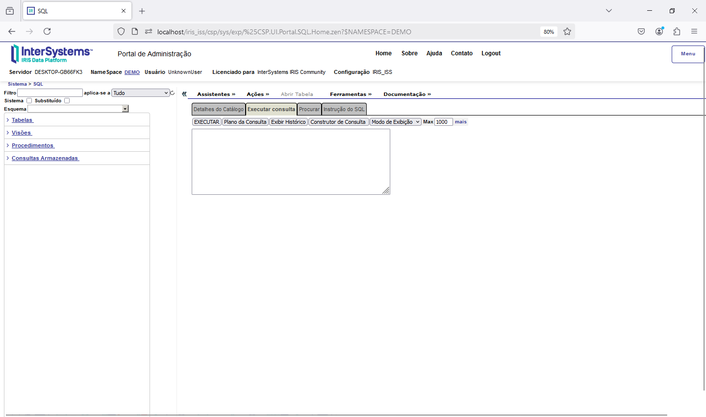
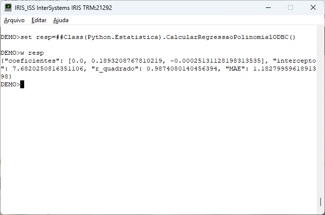
Executing our routine we have the information of the generated model:

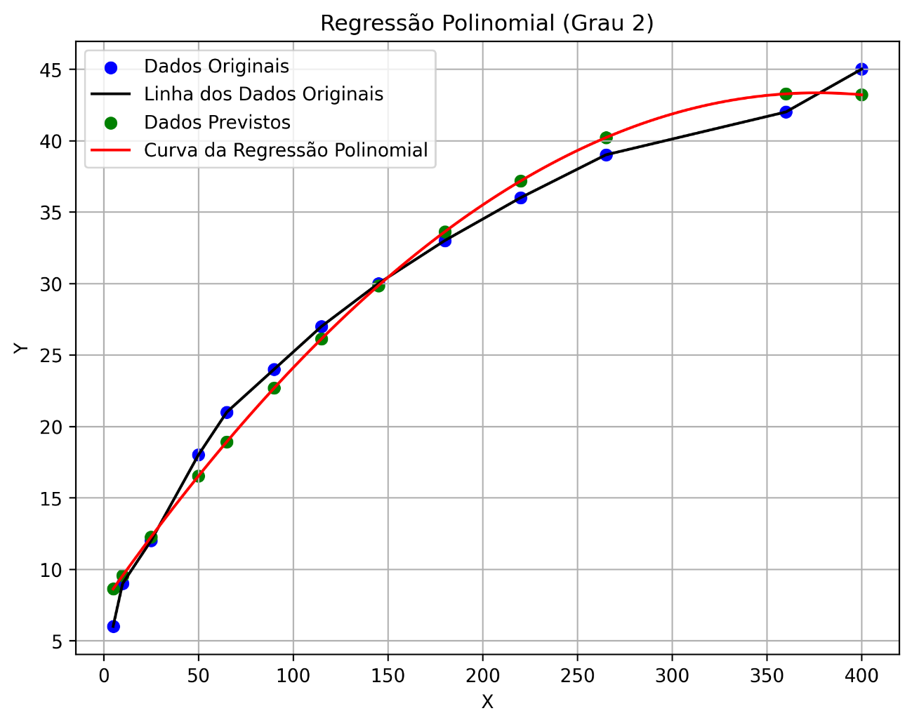
Our routine also generates a graph that gives us visual support for polynomial regression. Let's see how the graph turned out:

Another action we can take with the data that is now available is the use of Vector Search and RAG with the use of an LLM. To do this, we will vectorize the model of our table and from there ask LLM for some information.

For more information on using Vector Search in Iris, see the text available at https://www.intersystems.com/vectorsearch/

First, let's vectorize our table model. Below is the code with which we carry out this task:

ClassMethod IngestRelacional() As %String [ Language = python ]
{

    import json
    from langchain_iris import IRISVector
    from langchain_openai import OpenAIEmbeddings
    from langchain_text_splitters import RecursiveCharacterTextSplitter
    import iris    

    try:
    
        apiKey = iris.cls("Vector.Util").apikey()
        collectionName = "odbc_work"

        metadados_tabelas = [
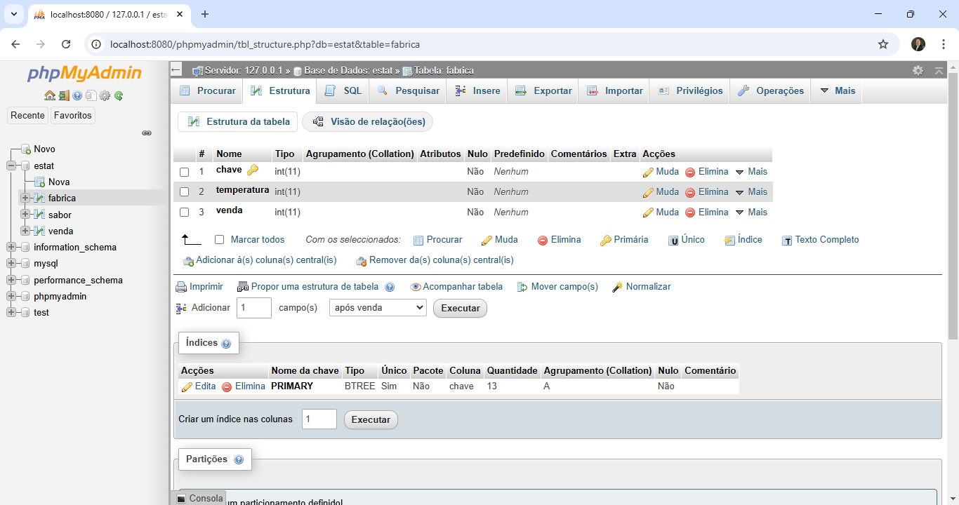
            "Tabela: estat.fabrica; Colunas: chave(INT), venda(INT), temperatura(INT)"
        ]
        
        text_splitter = RecursiveCharacterTextSplitter(chunk_size=2048, chunk_overlap=0)
        documents=text_splitter.create_documents(metadados_tabelas)
            
        # Vetorizar as definições das tabelas
        vectorstore = IRISVector.from_documents(
        documents=documents,
        embedding=OpenAIEmbeddings(openai_api_key=apiKey),
        dimension=1536,
        collection_name=collectionName
        )
        
        return json.dumps({"status": True})
    except Exception as err:
        return json.dumps({"error": str(err)})
}

Note that we don't pass the contents of the table to the ingest code, but its model. In this way, LLM is able, upon receiving the columns and their properties, to define an SQL according to our request.

This ingest code creates the odbc_work table that will be used to search for similarity in the table model, and then ask the LLM to return an SQL. For this we created a KEY API at OpenAI and used langchain_iris as a python library. For more details about the langchain_iris see the link https://github.com/caretdev/langchain-iris

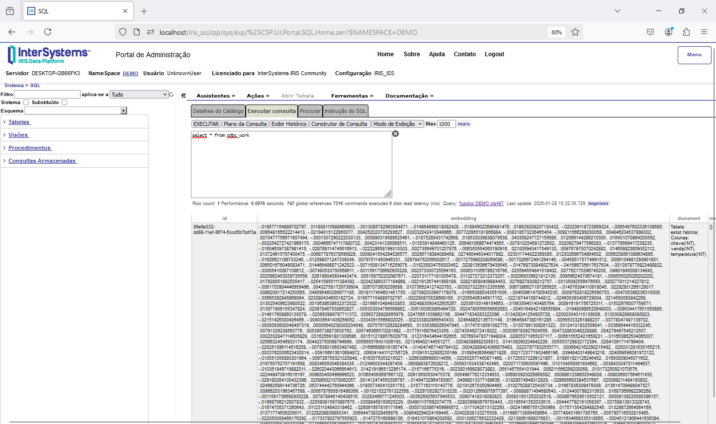
After ingest the definition of our table, we will have the odbc_work table  generated:

Now let's go to our third part, which is the access of a REST API that will consume the data that is vectorized to assemble a RAG.

See you later!