Internal Structure of Caché Database Blocks, Part 2
This text is a continuation of my article where I explained the structure a Caché database. In this article, I described the types of blocks, connections between them and their relation to globals. The article was purely theoretical. I made a project that helps visualize the block tree - and this article will explain how it works in great detail.

For demonstration purposes, I created a new database and cleared it of the globals that Caché initializes by default for all new databases. Let's create a simple global:
set ^colors(1)="red" set ^colors(2)="blue" set ^colors(3)="green" set ^colors(4)="yellow"

Note the image illustrating the blocks of the created global. This is a simple one, which is why we see its description in the type 9 block (globals catalog block). It is followed by the "upper and lower pointer" block (type 70), as the global tree isn't deep yet, and you can use a pointer to a data block still fitting into a single 8KB block.
Now, let's write so many values to another global that they will not fit into a single block - and we'll see new nodes in the pointer block pointing to new data blocks that could not fit into the first one.
Let's write 50 values, each 1000 characters long. Remember, the block size in our database is 8192 bytes.
set str=""
for i=1:1:1000 {
set str=str_"1"
}
for i=1:1:50 {
set ^test(i)=str
}
quitTake a look at the following image:

We have several nodes on the pointer block level pointing to data blocks. Each data block contains pointers to the next block ("right link"). Offset — points to the number of bytes occupied in this data block.
Let's try simulating a block split. Let's add so many values to the block that that the total block size exceeds 8KB, which will cause the block to be split in halves.
Sample code
set str=""
for i=1:1:1000 {
set str=str_"1"
}
set ^test(3,1)=str
set ^test(3,2)=str
set ^test(3,3)=strThe result can be seen below:
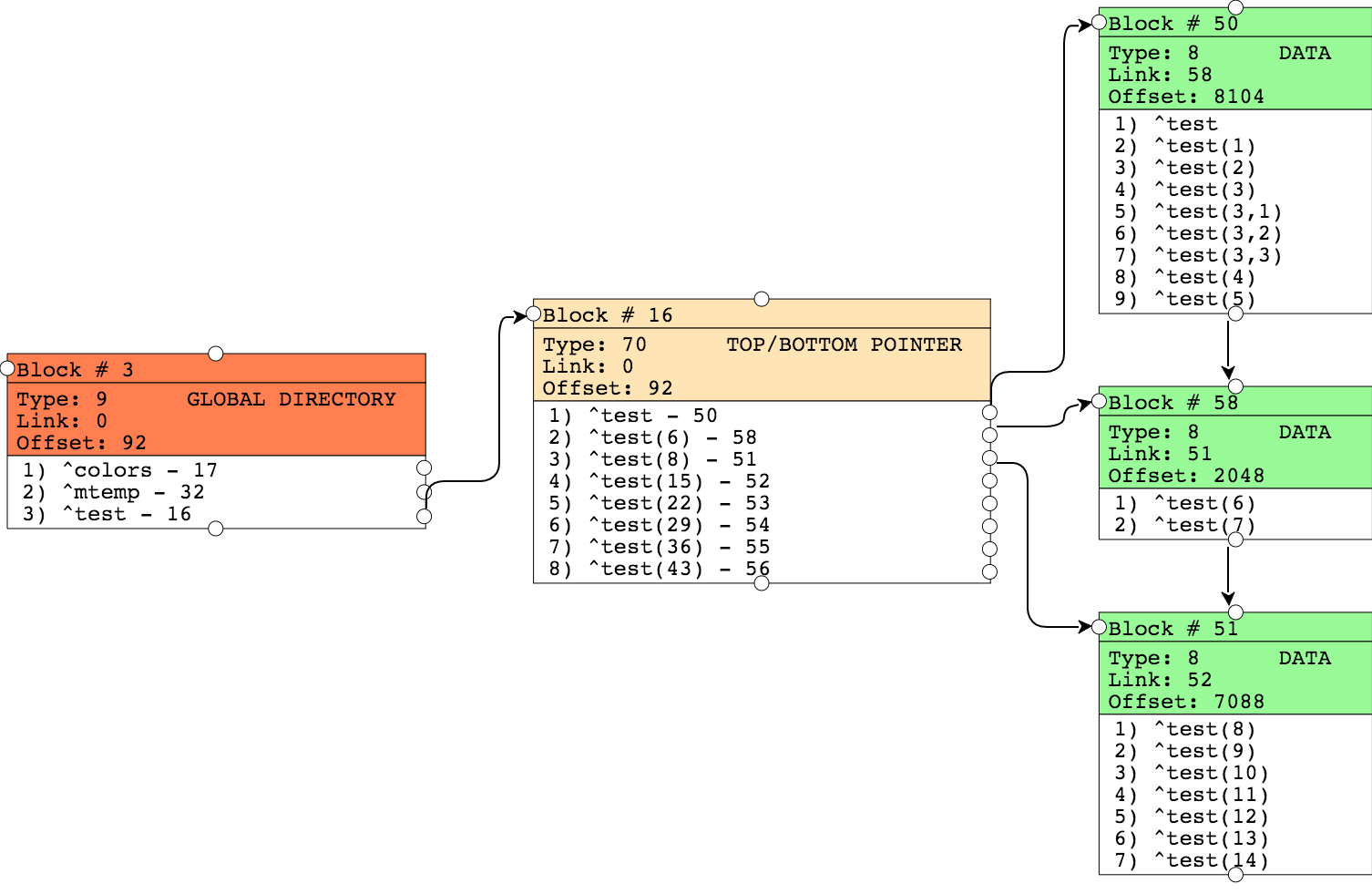
Block 50 is split and full of new data. The replaced values are now in block 58 and a pointer to this block now appears in the pointer block. Other blocks remained unchanged.
An example with long strings
If we use strings longer than 8KB (the size of the data block), we'll get blocks of "long data". We can simulate such a situation by writing strings as 10000 bytes, for instance.
Sample code
set str=""
for i=1:1:10000 {
set str=str_"1"
}
for i=1:1:50 {
set ^test(i)=str
}Let's look at the result:

As the result, the structure of blocks in the picture remained the same, since we did not add any new global nodes, but only changed values. However, the Offset value (number of bytes occupied) has changed for all blocks. For example, the Offset value for block #51 is now 172 instead of 7088. It's clear that now when the new value cannot fit in the block, the pointer to the last byte of data should be different, but where is our data? At the moment, my project doesn't support the possibility to show information about "large blocks". Let's use the ^REPAIR tool to get information about the new contents of block #51.

Let me elaborate on the way this tool works. We see a pointer to the right block #52, and the same number is specified in the parent pointer block in the next node. The global's collate is set to type 5. The number of nodes with long strings is 7. In some cases, the block can contain both data values for some nodes and long strings for others, all within a single block. We also see which next pointer reference should be expected at the beginning of the next block.
Regarding blocks of long strings: we see that the keyword "BIG" is specified as the global's value. It tells us that the data is actually stored in "big blocks". The same line contains the total length of the contained string, and the list of blocks storing this value. Let's take a look at the "block of long strings", block #73.
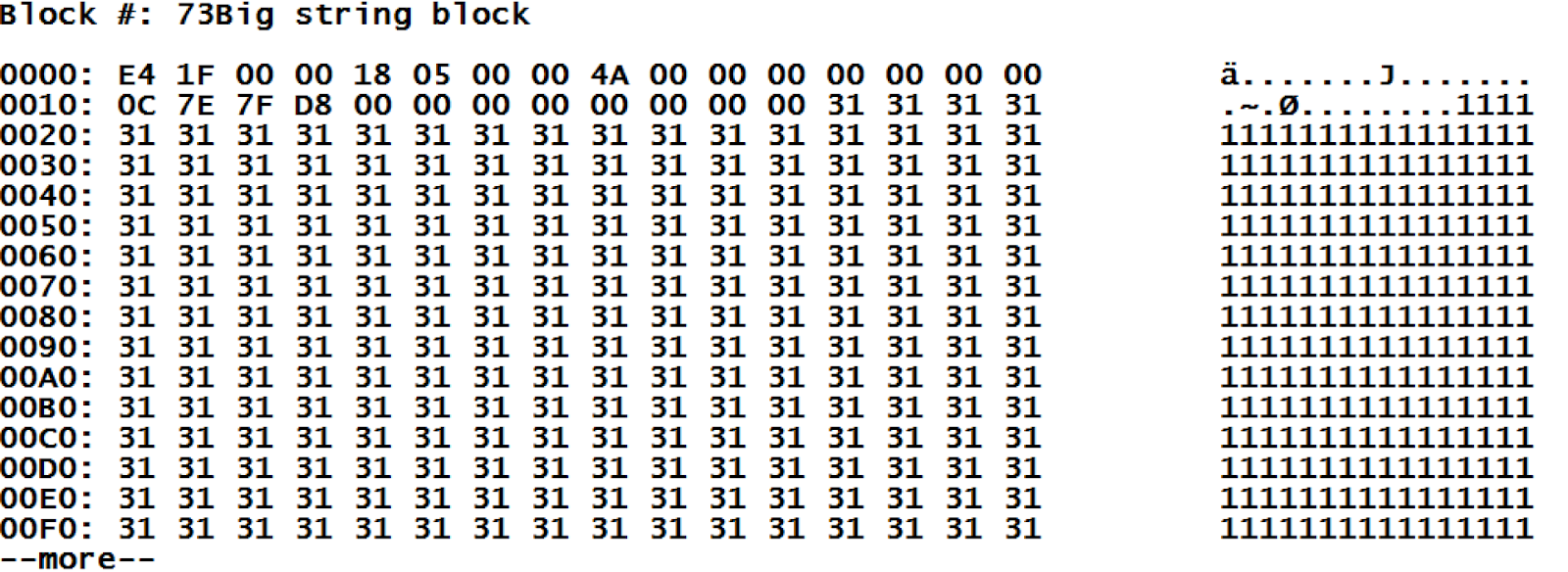
Unfortunately, this block is shown encoded. However, we can notice that the service information from the block header (which is always 28 bytes long) is followed by our data. Knowing the type of data makes the decoding of the header content quite easy:
|
Position |
Value |
Description |
Comment |
|
0-3 |
E4 1F 00 00 |
Offset pointing at the end of data |
We get 8164 bytes, plus 28 bytes of the header for a total of 8192 bytes, the block is full. |
|
4 |
18 |
Block type |
As we remember, 24 is the type identifier for long strings. |
|
5 |
05 |
Collate |
Collate 5 stands for “standard Caché” |
|
8-11 |
4A 00 00 00 |
Right link |
We get 74 here, as we remember that our value is stored in blocks 73 and 74 |
Let me remind you that the data in block 51 occupies just 172 bytes. This happened when we saved large values. So it looks like the block became almost empty with just 172 bytes of useful data, and yet it occupies 8kb! It is clear that in such a situation, the free space will be filled with new values, but Caché also allows us to compress such a global. For this purpose, the %Library.GlobalEdit class has the CompactGlobal method. To check the efficiency of this method, let’s use our example with a large volume of data – for instance, by creating 500 nodes.
Here is what we got.
kill ^test
for l=1000,10000 {
set str=""
for i=1:1:l {
set str=str_"1"
}
for i=1:1:500 {
set ^test(i)=str
}
}
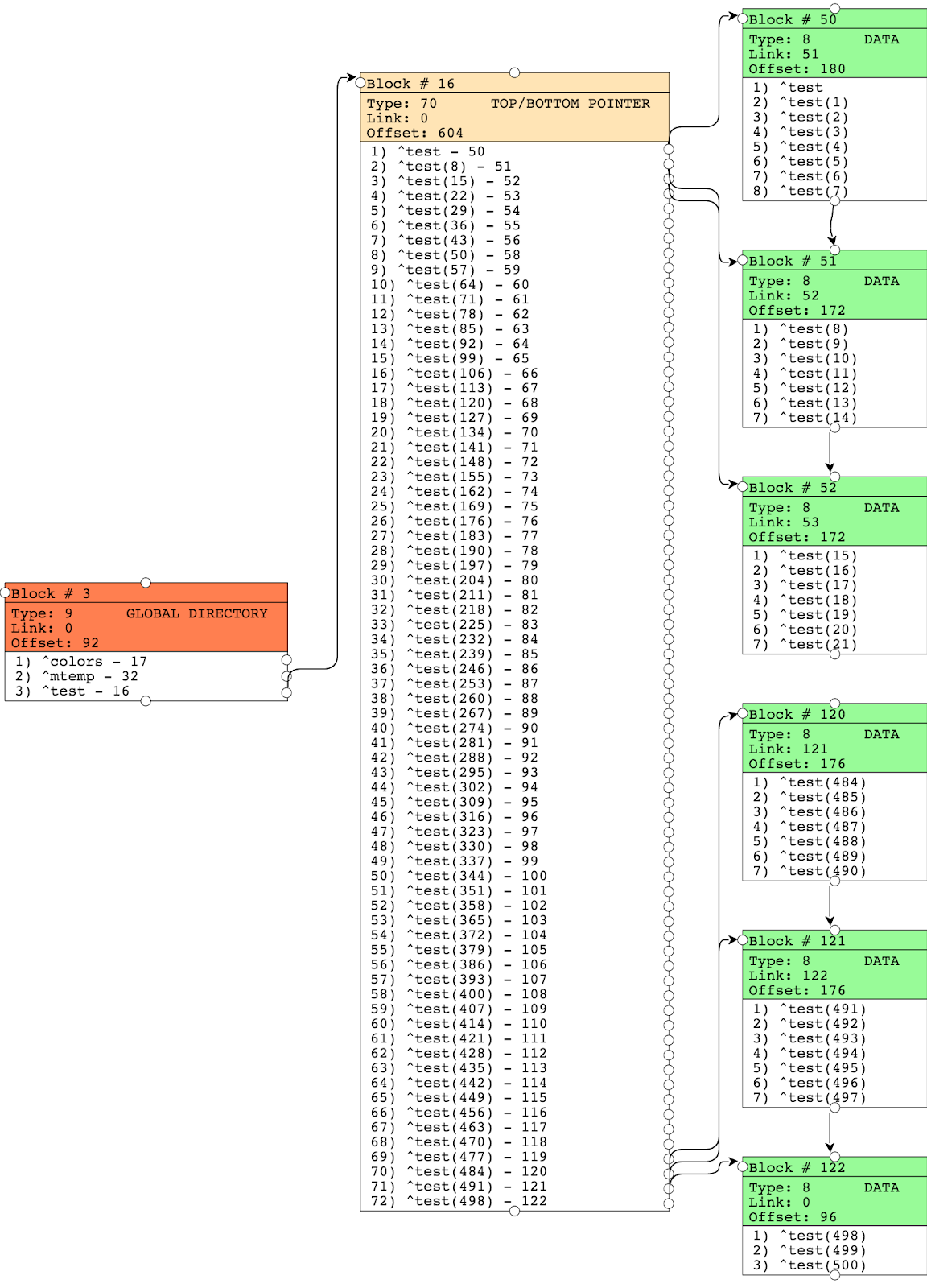
quitBelow we have show not all the blocks, but point should be clear. We have many of data blocks, but with small number of nodes.
Executing the CompactGlobal method:
write ##class(%GlobalEdit).CompactGlobal("test","c:\intersystems\ensemble\mgr\test")Let's take a look at the result. The pointers block now has just 2 nodes, which means that all our values went to two nodes, whereas we initially had 72 nodes in the pointer block. Therefore, we got rid of 70 nodes and thus reduced the data access time when going through the global, since it requires fewer block read operations.
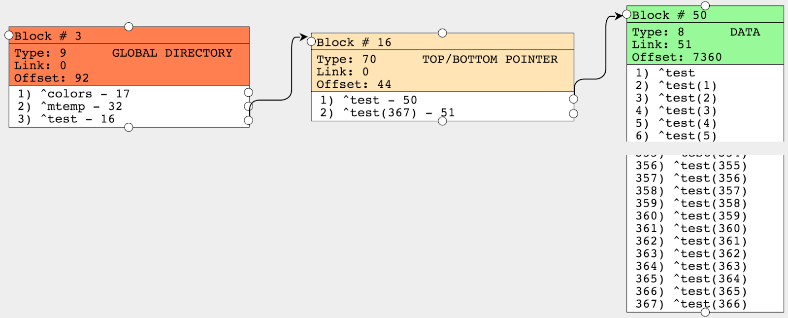
CompactGlobal accepts several parameters, such as the name of the global, the database and the target fill value, 90% by default. And now we see that Offset (the number of occupied bytes) equals 7360, which is around those 90%. Some output parameters of the function: the number of megabytes processed and the number of megabytes after compression. Previously, globals were compressed with the help of the ^GCOMPACT tool that is now considered obsolete.
It should be noted that a situation where blocks remain only partially filled is quite normal. Moreover, compression of globals may occasionally be undesirable. For example, if your global is mostly read and rarely modified, compression may come in handy. But if the global changes all the time, some sparsity in data blocks saves the trouble of having to split blocks too often, and the saving of new data will be faster.
In the next part of this article, I will go over another feature of my project that was implemented during at a first ever InterSystems hackathon at the InterSystems school 2015 – a map of database block distribution and its practical application.
Comments
You may try online demo here
Great article Dmitry. I think there's a minor typo under the dump of the big string block. You wrote:
Unfortunately, this block is shown unencrypted.
I think you mean "encrypted". Or perhaps better to say "encoded", and to refer to "decoding" in the subsequent sentence instead of "decryption".
Thanks for review, and I think you right, and fixed as you offer.