Run A Deep Learning Demo with Python3 Binding to HealthShare (Part II)

 

Keywords:   Jupyter Notebook, Tensorflow GPU, Keras, Deep Learning, MLP,  and HealthShare    

 

1. Purpose and Objectives

In  previous"Part I" we have set up a deep learning demo environment. In this "Part II" we will test what we could do with it.

Many people at my age had started with the classic MLP (Multi-Layer Perceptron) model. It is intuitive hence conceptually easier to start with.

So let's try a Keras "deep learning MLP" with standard demo data that everybody in AI/NN community has been using. It is a kind of so called "supervised learning". We will see how simple to run it on the Keras level.

We could later touch on its history and on why it's called "deep learning" the buzz word - what actually evolved over the recent 20 years. 

In the end I hope we could start to imagine or forecast a bit real use cases for it, since we have HealthShare along with us.

2. Scope and Disclaimer

We will try to 

• set up  a new Jupyter kernel for our tensorflow-gpu environment.
• define, train, and validate(test) a Keras MLP model with standard MNIST samples, like everyone else in ANN community.
• briefly talk its key parameters - only a few of them, fairly simple.
• briefly inspect the demo data - understanding the data is always the key in each and every experiment. 
• demo how easy it is to save some data sample into Cache / HealthShare, and to read it back for prediction (classification), and its implications.

Then we may rotate some test samples a bit to see how much we could confuse our trained model - then we may see its apparent limits.

We will skip the academic and mathematical part of it, but we might briefly talk into how it works.

Disclaimer:  MNIST data sample is publicly available for this demo purpose. Most demo code were cut to minimum and bare without error handling - all rely on the underlining components. The sources of the Keras codes will be listed in Acknowledgement.  The content will be revised anytime as needed.

 

3. Prerequisite

There is no prerequisite for the following experiments other than you need to set up the demo environment as listed in previous "Part I" article. 

 

4. Set up Jupyter Notebook

I ran the following commands in my previously installed "tensorflow-gpu" environment. 

(tensorflow-gpu) C:\>conda install ipykernel
Solving environment: done

... ...

(tensorflow-gpu) C:\>python -m ipykernel install --user --name tensorflow-gpu --display-name "Tensorflow-GPU"
Installed kernelspec tensorflow-gpu in C:\Users\zhongli\AppData\Roaming\jupyter\kernels\tensorflow-gpu

By doing so I created a new Jupyter kernel called e.g. "Tensorflow-GPU".

Now we can start the Jupyter Notebook from Anaconda Prompt as below:

(tensorflow-gpu) C:\anaconda3\keras\Zhong>jupyter notebook
[... ... 
[I 10:58:12.728 NotebookApp] The Jupyter Notebook is running at:
[I 10:58:12.729 NotebookApp] http://localhost:8889/?token=6b40f6e6749e88b80a338eec3330d06c181ead9b644...
[I 10:58:12.734 NotebookApp] Use Control-C to stop this server and shut down all kernels (twice to skip confirmation).
[C 10:58:12.835 NotebookApp] ... ... 

You will see its browser UI is started as below. If you click New... then open a new tab of "Tensorflow_GPU".

5. Train a Deep Learning MLP model

Let's try a standard deep learning MLP  model demo.

 5.1 Test the environment

Rename the Jupyter tab to something like "MLP_Demo_ HS", and test Python in its Cell [1] by running a line blow, then click "Run"

print('Hello World!')

Hello World!

 

5.2 Test Python Connection into a HealthShare 

Run a Python sample program in Cell[2] to test we still can connect into the HealthShare db instance as listed in "Part I" article.

import codecs, sys
import intersys.pythonbind3

try:
    print ("Simple Python binding sample")

    port = input("Cache server port (default 56778)? ")
    port = port.rstrip()
    if (port == ""):
        port = "56778"

    url = "localhost["+port+"]:SAMPLES"
    print ("Connection string: " + url)

    print ("Connecting to Cache server")
    conn = intersys.pythonbind3.connection( )
    conn.connect_now(url, "_SYSTEM", "SYS", None)
    print ("Connected successfully")

    print ("Creating database")
    database = intersys.pythonbind3.database( conn)

    print ("Opening Sample.Person instance with ID 1 with default concurrency and timeout")
    person = database.openid( "Sample.Person", "1", -1, -1)

    print ("Getting the value of the Name property")
    name = person.get("Name")
    print ("Value: " + name)

    print ("Test completed successfully")
except intersys.pythonbind3.cache_exception( err):
    print ("InterSystems Cache' exception")
    print (sys.exc_type)
    print (sys.exc_value)
    print (sys.exc_traceback)
    print (str(err))

Simple Python binding sample
Cache server port (default 56778)?
Connection string: localhost[56778]:SAMPLES
Connecting to Cache server
Connected successfully
Creating database
Opening Sample.Person instance with ID 1 with default concurrency and timeout
Getting the value of the Name property
Value: Zevon,Mary M.
Test completed successfully

 

5.3 Explanation - MLP model topology and MNIST data set

 

MLP network's topology is straightforward, as shown below. It normally has 1x input and 1x output layer, and has a number of hidden layers. 

Each layer has a number of neurons (nodes). Each neuron has an activation function. There can be fully meshed connections (called "Dense" model) between neurons on 2 different layers, as below. 

 

Correspondingly, the Keras MLP model we are testing below will have e.g.

• an input layer of  784 = 28 x 28 nodes  (so it represent a small image of 28x28 pixels; each will be a handwritten digit from "0" to "9"  - and the MNIST dataset contains 60,000 such images for training, and another 10,000 for testing)
• an output layer  of 10x nodes (each representing a classification result, between 0 and 9,  of an input image )
• 2x hidden layers, each having 512x nodes.

That's the key topology of this demo model. We will skip other details for now and go to have a run with it. 

 

 

5.4. Load MNIST sample data from Google Public Cloud    

Now we start to create the above model from very beginning,  by loading the Keras packages and MNIST data into a Jupyter Cell.  Then we will click "Run" button on the menu:

### Import Keras modules 
import keras
from keras.datasets import mnist
from keras.models import Sequential
from keras.layers import Dense, Dropout
from keras.optimizers import RMSprop

### Define key training parameter
batch_size = 128  # weights adjusted in 128 steps
num_classes = 10  # 10 classification results on the output layer
epochs = 20       # run the set of samples 20 times.

###load the data from Google public cloud 
# load the MNIST sample image  data, split between train and test sets
(x_train, y_train), (x_test, y_test) = mnist.load_data()

Note: if there are issues then follow the exception (more likely can't find a package etc), search Google for answers (99% chance you will get the answer), or post your question below.

The last line of code loaded the whole date set of 60,000 and 10,000 into a Python array of 3-dimension integers.  Let's load one of the training sample into HealthShare database to have a look.

 

5.5 Load a data sample into HealthShare globals.

In HealthShare -> SAMPLES namespace- > Sample.Person.cls, I scratch up this simplest class method:

ClassMethod SetTrainGlobals(d1 As %Integer = 0, d2 As %Integer = 0, value As %String = "", target As %String = "") As %BigInt [ SqlProc ]
{
Set ^XTrainInput(d1, d2) = value
Set ^YTrainTarget(d1) = target
return $$$OK
}

It will take an input training sample as a string into a global ^XTrainInput, and will save the input training target into ^YTrainTarget.

Let's recompile, refresh the connection per section 5.2, then run the call from the Python's cell as below:

result1 = person.run_obj_method("SetTrainGlobals", [0, 2, str(x_train[0]), str(y_train[0])])

On HealthShare -> Samples, you will see a global called ^XTrainGlobal(0, 2) was created with a string of 2D integers.

Later we can do another simple method to read the data back into a Python variable as a sample.  

 

5.6 Define the model and run the training

Let's finish off the MLP model definition and training in Jupyter.

Basically the code below, "reshape" just converts each 28 x 28 sample into a line of 1x 784 values, each between 0 and 255, then it is normalised to float type between 0 and 1.0.

Code between Model.Sequential and Model.Summary is to define a MLP of 784 x 512 x 512 x 10 nodes, with a "relu" activation function. 

Finally model.fit to train it and model.evalute to assess the test result.   

x_train = x_train.reshape(60000, 784)
x_test = x_test.reshape(10000, 784)
x_train = x_train.astype('float32')
x_test = x_test.astype('float32')
x_train /= 255
x_test /= 255

print(x_train.shape[0], 'train samples')
print(x_test.shape[0], 'test samples')

# convert class vectors to binary class matrices
y_train = keras.utils.to_categorical(y_train, num_classes)
y_test = keras.utils.to_categorical(y_test, num_classes)

model = Sequential()
model.add(Dense(512, activation='relu', input_shape=(784,)))
model.add(Dropout(0.2))
model.add(Dense(512, activation='relu'))
model.add(Dropout(0.2))
model.add(Dense(num_classes, activation='softmax'))

model.summary()

model.compile(loss='categorical_crossentropy',
              optimizer=RMSprop(),
              metrics=['accuracy'])

history = model.fit(x_train, y_train,
                    batch_size=batch_size,
                    epochs=epochs,
                    verbose=1,
                    validation_data=(x_test, y_test))

score = model.evaluate(x_test, y_test, verbose=1)

print('Test loss:', score[0])
print('Test accuracy:', score[1])

Using TensorFlow backend.

60000 train samples
10000 test samples
_________________________________________________________________
Layer (type)                 Output Shape              Param #
=================================================================
dense_1 (Dense)              (None, 512)               401920
_________________________________________________________________
dropout_1 (Dropout)          (None, 512)               0
_________________________________________________________________
dense_2 (Dense)              (None, 512)               262656
_________________________________________________________________
dropout_2 (Dropout)          (None, 512)               0
_________________________________________________________________
dense_3 (Dense)              (None, 10)                5130
=================================================================
Total params: 669,706
Trainable params: 669,706
Non-trainable params: 0
_________________________________________________________________
Train on 60000 samples, validate on 10000 samples
Epoch 1/20
60000/60000 [==============================] - 11s 178us/step - loss: 0.2476 - acc: 0.9243 - val_loss: 0.1057 - val_acc: 0.9672
Epoch 2/20
60000/60000 [==============================] - 6s 101us/step - loss: 0.1023 - acc: 0.9685 - val_loss: 0.0900 - val_acc: 0.9730
Epoch 3/20
60000/60000 [==============================] - 6s 101us/step - loss: 0.0751 - acc: 0.9780 - val_loss: 0.0756 - val_acc: 0.9783
Epoch 4/20
60000/60000 [==============================] - 6s 100us/step - loss: 0.0607 - acc: 0.9816 - val_loss: 0.0771 - val_acc: 0.9801
Epoch 5/20
60000/60000 [==============================] - 6s 101us/step - loss: 0.0512 - acc: 0.9844 - val_loss: 0.0761 - val_acc: 0.9810
Epoch 6/20
60000/60000 [==============================] - 6s 102us/step - loss: 0.0449 - acc: 0.9866 - val_loss: 0.0747 - val_acc: 0.9809
Epoch 7/20
60000/60000 [==============================] - 6s 101us/step - loss: 0.0377 - acc: 0.9885 - val_loss: 0.0765 - val_acc: 0.9811
Epoch 8/20
60000/60000 [==============================] - 6s 101us/step - loss: 0.0334 - acc: 0.9898 - val_loss: 0.0774 - val_acc: 0.9840
Epoch 9/20
60000/60000 [==============================] - 6s 101us/step - loss: 0.0307 - acc: 0.9911 - val_loss: 0.0771 - val_acc: 0.9842
Epoch 10/20
60000/60000 [==============================] - 6s 105us/step - loss: 0.0298 - acc: 0.9911 - val_loss: 0.1015 - val_acc: 0.9813
Epoch 11/20
60000/60000 [==============================] - 6s 102us/step - loss: 0.0273 - acc: 0.9922 - val_loss: 0.0869 - val_acc: 0.9833
Epoch 12/20
60000/60000 [==============================] - 6s 99us/step - loss: 0.0247 - acc: 0.9926 - val_loss: 0.0945 - val_acc: 0.9824
Epoch 13/20
60000/60000 [==============================] - 6s 101us/step - loss: 0.0224 - acc: 0.9935 - val_loss: 0.1040 - val_acc: 0.9823
Epoch 14/20
60000/60000 [==============================] - 6s 100us/step - loss: 0.0219 - acc: 0.9939 - val_loss: 0.1038 - val_acc: 0.9835
Epoch 15/20
60000/60000 [==============================] - 6s 104us/step - loss: 0.0227 - acc: 0.9936 - val_loss: 0.0909 - val_acc: 0.9849
Epoch 16/20
60000/60000 [==============================] - 6s 100us/step - loss: 0.0198 - acc: 0.9944 - val_loss: 0.0998 - val_acc: 0.9826
Epoch 17/20
60000/60000 [==============================] - 6s 101us/step - loss: 0.0182 - acc: 0.9951 - val_loss: 0.0984 - val_acc: 0.9832
Epoch 18/20
60000/60000 [==============================] - 6s 102us/step - loss: 0.0178 - acc: 0.9955 - val_loss: 0.1150 - val_acc: 0.9839
Epoch 19/20
60000/60000 [==============================] - 6s 100us/step - loss: 0.0167 - acc: 0.9954 - val_loss: 0.0975 - val_acc: 0.9847
Epoch 20/20
60000/60000 [==============================] - 6s 102us/step - loss: 0.0169 - acc: 0.9956 - val_loss: 0.1132 - val_acc: 0.9832
10000/10000 [==============================] - 1s 71us/step
Test loss: 0.11318948425535869
Test accuracy: 0.9832 

 

That's all - now it's "trained". Only a few line of codes, this Keras deep learning MLP runs fairly efficiently on our "tensorflow-gpu" environment. It validates all of our kit installation so far. 

 

6 Test the model with a sample

Let's test the trained model with a specified sample below.

We will randomly select a specific sample out of the 10,000 x_test set, and save it into another HealthShare global,  then read it back out of the global into a Python array as a demo sample. We will test the trained model with it.

Then we will rotate this input sample 90, 180 and 270 degrees, and re-test our model , to see whether we would confuse it . 

 

6.1 Save a sample into HealthShare - Demo 

Let's randomly pick a sample, say the 12th out of the 10,000 test samples, and save it into a HS global:

Add a new class method in HealthShare -> SAMPLE -> Sample.Person class:

ClassMethod SetT2Globals(d1 As %Integer = 0, d2 As %Integer = 0, d3 As %Integer = 0, value As %String = "", target As %String = "") As %BigInt [ SqlProc ]
{
         Set ^XTestInput(d1, d2, d3) = value
         Set ^YTestTarget(d1, d2) = target
         return $$$OK
}

Recompile Sample.Person.cls.  In Jupyter Notebook, re-run Section 5.2 code to refresh the db binding; then run this line to save the sample of 28 x 28 numbers into global ^XTestInput:

import re
n = 12  # randomly choose a sample 
for i in range(0, len(x_train[n])):
     r1 = person.run_obj_method("SetT2Globals", [1, n, i, re.sub('0\s0', '  0   0', str(x_test[n][i])), str(y_test[n])])

Now we can see a sample of 2D array was saved into a HS SAMPLE global ^XTestInput. Each number is a pixel grey scale of 0-255. From below the HS Management Portal we can easily "tell" it's a "9":

   

6.2 Read a sample out of HealthShare global- Demo

We can certainly read the sample out of a HS database global.  

Add another class method into Sample.Person.cls, and recompile it

ClassMethod GetT2Globals(d1 As %Integer = 0, d2 As %Integer = 0, d3 As %Integer = 0) As %String [ SqlProc ]
{
     Set value = ^XTestInput(d1, d2, d3)
     return value
}

In Jupyter, refresh the DB binding as above, then run this Python code to read the global out of HealthShare as a string, re-format it, then convert it to a 1 x 2D number array:

import re, ast
sample = ""
for i in range(0, len(x_train[n])):
   sample += person.run_obj_method("GetT2Globals", [1, n, i])
#convert it to numpy ndarray
as1  = np.array(ast.literal_eval(re.sub('\s+', ',', re.sub('0\]', '0', re.sub('\[  ', '', re.sub('\]\[', ' ', sample))))))   
Sample12 = as1.reshape(1, 28, 28)
print(Sample12)

 

6.3 Test our trained model 

We can now send this array "Sample12" into the trained model on Jupyter.  model.predict and/or model.predict_classes does the job for us:

Sample12  = Sample12.reshape(1, 784)
Sample12f = Sample12.astype('float32')/255  # normalise it to float between [0, 1]
Result12f = model.predict(Sample12f)   #test the 1x784 sample, the result is a 1d matrix
print(Result12f)

Result12 = model.predict_classes(Sample12f)  #test the sample, the result is a clasified lable.
print(Result12)

[[2.5672970e-27 1.1168821e-25 1.3736557e-20 6.2964843e-17 7.0107062e-09 6.2905544e-17 1.5294099e-28 7.8019199e-17 3.5748028e-16 1.0000000e+00]]
[9]

The result indicated that the neuron #9 on the output layer has the maximum value of  "1.0", so the classification result is "9".  It's a correct result.

We can certainly send any man-made sample(s) of 28 x 28 integers into the model to have a try.

 

6.4 Rotate our sample to re-test our model?

How about this - could we rotate this sample 90 degree anticlockwise to have another try? 

Sample12 = Sample12.reshape(28, 28)  #reshape to 2D array values
Sample1290 = np.rot90(Sample12)  #rotate in 90 degree
print(Sample1290)

Then we re-test our model:

Sample12901  = Sample1290.reshape(1, 784)
Sample1290f = Sample12901.astype('float32')/255  
Result1290f = model.predict(Sample1290f)   
print(Result1290f)

Result1290 = model.predict_classes(Sample1290f)  
print(Result1290)

[[2.9022769e-05 1.2192334e-20 1.7143857e-07 3.0004558e-11 2.4583075e-11 6.2443775e-01 2.5749558e-05 3.7550735e-01 2.0722151e-08 5.5368415e-10]]
[5]

Ok, now our model believes it's a "5" - neuron #5 was triggered with the maximum output value.  It's slightly confused! (Can be pardoned since it does look like a 5 in its up-right part).

Let's turn our sample again to 180 degree - what would our model think?  

[[3.3131425e-11 3.0135434e-27 8.7524540e-23 7.1371946e-24 2.4029167e-13 4.2327470e-09 1.0000000e+00 1.7086377e-18 1.3129146e-18 2.8595145e-22]]
[6]

No mistake, of course it's identified to a "6"!  We human will tell it as a "6" instead of "9". 

Let's turn it the last time to 270 degrees: 

Apparently, it's confused again - it is recognised to be a "4"

[[1.6130849e-06 3.0311636e-14 2.1490927e-03 2.7108688e-03 9.9499077e-01 1.4130991e-04 6.2298268e-06 8.6649310e-09 2.9320630e-12 1.5710594e-07]]
[4]

 

6.5 Compared with public cloud tools?

I exported the above array via a line of Python code into a PNG, then rotate it, flip it, and put them together on an image. It would look like this:

 

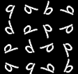
Now I upload it separately into "Google Vision API", "Amazon Rekognition", and "Microsoft Computer Vision API", what would be the results?

Well, it seems that AWS has the slightly best score of 95% on "number" in this case (this is certainly not meant to be a representative result). 

1. Google Vision API results:

 

2. AWS Rekognition Results

3. Microsoft Computer Vision: 

 

7. What's next

Next, we will follow up on a few other quick points such as 

• How MLP works in a nutshell?
• Limits and possible use cases?
• A quick walkthrough on most common ML/DL/ANN models that can be running on the current stacks.  
• Acknowledgements