Understanding SQL Window Functions (Part 3)

Article

José Pereira · 4 hr ago 12m read

In this final part of our introduction to Window Functions, we will explore the remaining functions that have not been covered yet. You will also discover performance tips and a practical guide to help you decide when (and when not) to use window functions effectively.

1. Offset and Positional Value Functions

Overview

These functions reference values are calculated from other rows relative to the current row, or they are extracted from the first, last, or nth values within a window.

LAG(column, offset, default) — retrieves the value offset from the preceding row.
LEAD(column, offset, default) — recovers the value offset from the subsequent rows.
FIRST_VALUE(column) — returns the first value in the window frame.
LAST_VALUE(column) — returns the last value in the window frame.
NTH_VALUE(column, n) — returns the nth value in the window frame.

All of them are essential for comparing the current row to others in the same sequence.

Example 1 — Patient Cholesterol Trends

Let’s analyze how each patient’s cholesterol levels evolve across multiple visits.

CREATE TABLE LabResults (
    PatientID INTEGER,
    VisitDate DATE,
    Cholesterol INTEGER
)

INSERT INTO LabResults
SELECT 1,'2024-01-10',180 UNION ALL
SELECT 1,'2024-02-15',195 UNION ALL
SELECT 1,'2024-03-20',210 UNION ALL
SELECT 2,'2024-01-12',160 UNION ALL
SELECT 2,'2024-03-10',155 UNION ALL
SELECT 2,'2024-04-15',165

We need to:

Use LAG() to retrieve the previous cholesterol value for each patient.
Calculate the change in cholesterol between visits (Delta).
Use FIRST_VALUE() to capture each patient’s baseline cholesterol.
Compute the percentage change from baseline with PercentChange.
Order the final result by PatientID and VisitDate.

SELECT
    PatientID,
    VisitDate,
    Cholesterol,
    LAG(Cholesterol) OVER (PARTITION BY PatientID ORDER BY VisitDate) AS PrevValue,
    Cholesterol - LAG(Cholesterol) OVER (PARTITION BY PatientID ORDER BY VisitDate) AS Delta,
    FIRST_VALUE(Cholesterol) OVER (PARTITION BY PatientID ORDER BY VisitDate) AS Baseline,
    ROUND(
        100.0 * Cholesterol /
        FIRST_VALUE(Cholesterol) OVER (PARTITION BY PatientID ORDER BY VisitDate), 2
    ) AS PercentChange
FROM LabResults
ORDER BY PatientID, VisitDate

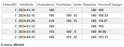Fig 1 - Patient Cholesterol Trends

This data helps us to the following key findings:

Patient 1 shows a consistent upward trend: cholesterol increased from 180 to 210 over three visits, with each step rising by 15 units and a cumulative percent change of +16.67% from baseline.
Patient 2 exhibits a fluctuating pattern: initial drop from 160 to 155 (−5 units, −3.13%), followed by a rebound to 165 (+10 units, +6.25%), resulting in a net increase of +3.13% from baseline.
Patient 1’s cholesterol rose steadily, suggesting a progressive change that may warrant monitoring or intervention.
Patient 2’s cholesterol varied but remained close to baseline, indicating less consistent but relatively stable levels.

👉 Why it is useful: Detecting trends or sudden changes in patient lab results is ideal for monitoring chronic conditions or treatment effectiveness.

Example 2 — Inventory Trend Analysis with Look-Ahead and Historical Benchmarks

Let's analyze the evolution of each product's inventory history by comparing the current stock against the projected stock for the next day (using LEAD) to calculate daily usage and set a historical reorder threshold based on the stock from three days before (with NTH_VALUE).

CREATE TABLE InventoryLog (
    LogDate DATE,
    ProductID VARCHAR(10),
    InventoryCount INT
)

INSERT INTO InventoryLog (LogDate, ProductID, InventoryCount)
SELECT '2025-11-01', 'A101', 500 UNION ALL
SELECT '2025-11-02', 'A101', 480 UNION ALL
SELECT '2025-11-03', 'A101', 450 UNION ALL
SELECT '2025-11-04', 'A101', 400 UNION ALL
SELECT '2025-11-05', 'A101', 350 UNION ALL
SELECT '2025-11-06', 'A101', 300 UNION ALL
SELECT '2025-11-07', 'A101', 250 UNION ALL
SELECT '2025-11-08', 'A101', 200 UNION ALL
SELECT '2025-11-01', 'B202', 120 UNION ALL
SELECT '2025-11-02', 'B202', 115 UNION ALL
SELECT '2025-11-03', 'B202', 110 UNION ALL
SELECT '2025-11-04', 'B202', 100

We need to:

Use LEAD(InventoryCount, 1) to retrieve the stock count of the next chronological log date.
Calculate the daily usage by subtracting the LEAD stock count from the current InventoryCount.
Use NTH_VALUE(InventoryCount, 3) within a window defined from the beginning to the current row (ROWS BETWEEN UNBOUNDED PRECEDING AND CURRENT ROW) to retrieve the inventory count from the third recorded day.

SELECT
    LogDate,
    ProductID,
    InventoryCount AS Current_Stock,

    LEAD(InventoryCount, 1) OVER (
        PARTITION BY ProductID
        ORDER BY LogDate
    ) AS Next_Day_Stock,

    InventoryCount - LEAD(InventoryCount, 1) OVER (
        PARTITION BY ProductID
        ORDER BY LogDate
    ) AS Daily_Usage,

    NTH_VALUE(InventoryCount, 3) OVER (
        PARTITION BY ProductID
        ORDER BY LogDate
        ROWS BETWEEN UNBOUNDED PRECEDING AND CURRENT ROW
    ) AS Stock_Three_Days_Ago_Threshold
FROM
    InventoryLog
ORDER BY
    ProductID, LogDate;

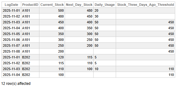Fig 2 - Inventory Trend Analysis with Look-Ahead and Historical Benchmarks

This data allows us to identify the following key findings:

The daily usage of product A101 initially increased from 20 units to 30 units, and then stabilized at a consistent 50 units per day from November 3rd to November 7th.
For the data points where the window has at least three rows (starting on 2025-11-03), the reorder threshold is established as the stock from three days prior.
As of 2025-11-05, the current stock of 350 for A101 is significantly below the historical benchmark of 450, indicating a potential need for replenishment soon.

👉 Why it is useful: The LEAD() function provides future context by showing the subsequent value in a time series, which is essential for calculating rates of change (e.g., daily usage). The NTH_VALUE() function allows analysts to establish dynamic, indexed benchmarks within a rolling window (e.g., comparing the current value against the value from the start of the week or a specific historical point) for proactive decision-making.

2. Moving and Cumulative Window Functions

Overview

These functions use explicit frame clauses (ROWS BETWEEN ...) to compute metrics over a sliding or cumulative subset of rows.

Typical aggregates:

SUM() or AVG() for rolling totals or averages.
Any aggregate function can operate over a bounded or unbounded frame.

Typical syntax:

SUM(value) OVER (  
    PARTITION BY ...
    ORDER BY ...
    ROWS BETWEEN n PRECEDING AND CURRENT ROW
)

Example 1 — Rolling Account Balances

Let’s analyze how each account’s transaction history evolves using rolling and cumulative metrics.

CREATE TABLE Transactions (
    AccountID INTEGER,
    TxDate DATE,
    Amount INTEGER
)

INSERT INTO Transactions
SELECT 1001,'2024-01-01',100 UNION ALL
SELECT 1001,'2024-01-05',250 UNION ALL
SELECT 1001,'2024-01-07',150 UNION ALL
SELECT 1001,'2024-01-10',300 UNION ALL
SELECT 1002,'2024-01-02',500 UNION ALL
SELECT 1002,'2024-01-06',400 UNION ALL
SELECT 1002,'2024-01-09',600

We need to complete the next steps:

Use SUM() with a window frame of ROWS BETWEEN 2 PRECEDING AND CURRENT ROW to calculate a 3-transaction moving sum (MovingSum).
Use AVG() with ROWS BETWEEN UNBOUNDED PRECEDING AND CURRENT ROW to compute a running average (RunningAvg) from the start of each account’s history.
Partition by AccountID and order by TxDate to track balances chronologically.
Display all transactions with the metrics calculated above.

SELECT
    AccountID,
    TxDate,
    Amount,
    SUM(Amount) OVER (
        PARTITION BY AccountID
        ORDER BY TxDate
        ROWS BETWEEN 2 PRECEDING AND CURRENT ROW
    ) AS MovingSum,
    AVG(Amount) OVER (
        PARTITION BY AccountID
        ORDER BY TxDate
        ROWS BETWEEN UNBOUNDED PRECEDING AND CURRENT ROW
    ) AS RunningAvg
FROM Transactions
ORDER BY AccountID, TxDate

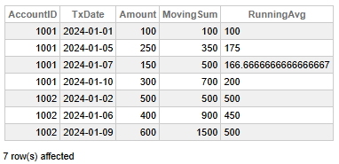Fig 3 - Rolling Account Balances

This data helps us conclude the following key findings:

Account 1001 displays a steady increase in transaction amounts over time, with a total MovingSum of 700 and a final RunningAvg of 200, indicating growing activity and a consistent upward trend.
Account 1002 has higher transaction values overall, reaching a MovingSum of 1500 and maintaining a stable RunningAvg of 500, suggesting larger but more balanced transactions.
Account 1002 contributes more in total volume despite fewer transactions, highlighting its higher value per transaction.

👉 Why it is useful: This method smooths fluctuations and clearly visualizes transaction trends, which is ideal for financial monitoring and forecasting.

Example 2 — COVID Cases Moving Average

Let’s track how daily COVID case counts evolved across regions using a rolling average to smooth short-term fluctuations.

CREATE TABLE CovidStats (
    Region VARCHAR(50),
    ReportDate DATE,
    Cases INTEGER
)

INSERT INTO CovidStats
SELECT 'North','2024-01-01',12 UNION ALL
SELECT 'North','2024-01-02',15 UNION ALL
SELECT 'North','2024-01-03',20 UNION ALL
SELECT 'North','2024-01-04',18 UNION ALL
SELECT 'North','2024-01-05',25 UNION ALL
SELECT 'South','2024-01-01',10 UNION ALL
SELECT 'South','2024-01-02',11 UNION ALL
SELECT 'South','2024-01-03',13 UNION ALL
SELECT 'South','2024-01-04',15

We should take the following steps:

Use AVG() with a window frame of ROWS BETWEEN 2 PRECEDING AND CURRENT ROW to calculate a 3-day moving average of COVID cases.
Partition by Region and order by ReportDate to compute trends independently for each region.
Display all daily case counts alongside their corresponding moving averages.

SELECT
    Region,
    ReportDate,
    Cases,
    AVG(Cases) OVER (
        PARTITION BY Region
        ORDER BY ReportDate
        ROWS BETWEEN 2 PRECEDING AND CURRENT ROW
    ) AS Moving3DayAvg
FROM CovidStats
ORDER BY Region, ReportDate

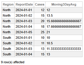Fig 4 - COVID Cases Moving Average

This data enables us to make the following key findings:

The North region exhibits a clear upward trajectory in daily cases, rising from 12 to 25 over five days, with the Moving 3-Day Average increasing steadily from 12 to 21.
The South region displays a moderate increase, with cases rising from 10 to 15, and the Moving 3-Day Average climbing from 10 to 13.
North’s higher Moving 3-Day Average values (peaking at 21) indicate a faster and more intense growth in cases compared to South.
North’s case acceleration is sharper, suggesting a need for closer monitoring or intervention, contrary to South's.

👉 Why it is useful: This method provides a clear trendline of increases or declines over time, making it ideal for public health monitoring and forecasting.

3. Performance & Optimization Tips

Specify the Window Frame: For aggregate functions (e.g., SUM()), use the smallest possible frame (e.g., ROWS BETWEEN 2 PRECEDING AND CURRENT ROW) to reduce calculation overhead per row.
Limit Data Early: Apply WHERE clauses in a CTE or subquery before the window function executes. This decreases the number of rows the function must process.
Maintain Statistics: Run TUNE TABLE regularly to keep statistics current, ensuring the Query Optimizer selects the optimal execution plan (e.g., utilizing your indexes).
Analyze the Plan: Always employ EXPLAIN to confirm that the optimizer is using an index for the sorting phase rather than performing a full sort.
Choose Simpler Functions: Opt for ROW_NUMBER() over RANK() or DENSE_RANK() when ties do not matter, since it is generally faster.
Use Existing Indexes: Check if an existing index already satisfies the PARTITION BY and ORDER BY requirements before creating a new one.
Consider creating a "POC" Index in cases where existing indexes are insufficient. A POC Index is an index that explicitly covers the columns in the following order: Partitioning (PARTITION BY), Ordering (ORDER BY), and Covering columns (any other columns referenced in the window function or select list). It eliminates costly table sorting (1, 2).

4. When to Use — and When Not To

✅ When to Use Window Functions	❌ When NOT to Use Window Functions
Calculating Running Totals or Cumulative Distributions. (e.g., running sum of sales over time).	Simple Row-Level Operations. If you simply need to calculate a value based on the current row's columns (e.g., column_A * column_B), standard arithmetic is enough.
Ranking Rows within a Group. (e.g., finding the top 5 students in each class with the help of the RANK(), DENSE_RANK(), or ROW_NUMBER()).	*Filtering/Aggregating the Entire* Dataset to a Single Row per Group. Apply the standard GROUP BY** clause for summarizing data (e.g., total sales per year).
Calculating Moving Averages or other Sliding Window Calculations. Defining a specific frame (e.g., the average of the last 3 days' sales).	You need to reduce the number of returned rows. Window functions calculate values but do not implicitly filter rows. When you need to limit results, utilize WHERE or a subquery/CTE with the window function.
Comparing a Row to a Preceding or Following Row. (e.g., calculating the day-over-day change in stock price with LAG() or LEAD()).	The calculation can be performed more easily and clearly with a JOIN or a simple CASE statement, which is more efficient for particular, straightforward lookups.
Calculating Percentiles/Quartiles or other Distribution Metrics. (e.g., finding the median salary utilizing NTILE() or PERCENT_RANK()).	Working with extensive, non-indexed datasets where performance is critical, and a simpler GROUP BY query could achieve the goal faster (though it is increasingly rare with modern database optimizers).

5. Final Thoughts

As we wrap up this three-part introduction to Window Functions, let’s take a moment to reflect on our journey:

Part 1 laid out the foundation by explaining the mechanics and syntax of window functions (how they work and what makes them different from standard aggregations).
Parts 2 and 3 focused on the most commonly used window functions, illustrated with practical analytical examples that show their real-world value.
Part 3 additionally introduced performance tips and a decision-making guide to help you determine when (and when not) to use window functions.

Window functions significantly enhance the analytical power of SQL, allowing you to express complex logic in an elegant, simple, and maintainable way. They also often replace convoluted procedural code and/or multi-step aggregations.

Throughout the series, we grouped the functions into logical categories to help you better understand their roles and simplify memorization. We hope this structure proves to be practical for both learning and future reference.

The performance tips shared in Part 3 can assist you in avoiding common pitfalls and ensure your queries run smoothly.

The usage guide provides a practical framework for determining when window functions are the right tool, and when simpler alternatives may be more suitable.

We hope that this series facilitated your understanding of the power and versatility of window functions. If you found this beneficial, have any questions, feedback, or insights you wish to share, we would love to hear from you. Your thoughts can make the learning journey richer for everyone.

This article was written with the help of AI tools to clarify concepts and improve readability.