Understanding SQL Window Functions (Part 2)

Article

José Pereira · 8 hr ago 10m read

#Analytics #Performance #SQL #Tools #InterSystems IRIS

In Part 1, we explored how window functions operate. We learned the logic behind PARTITION BY, ORDER BY, and such functions as ROW_NUMBER() and RANK(). Now, in Part 2, let's delve into more window functions with practical examples.

1. Aggregate-over-Window Functions

Overview

These functions compute an aggregate (e.g., sum, average, min, max, count, etc.) over the defined window frame but don’t collapse rows.
Each row remains visible, augmented with aggregated values for its partition.

Supported functions include the following:

AVG() — average of values in the window frame.
SUM() — total of values in the window frame.
MIN() — minimum value.
MAX() — maximum value.
COUNT() — number of rows or non-NULL values.

Syntax:

function(...) OVER (PARTITION BY ... ORDER BY ...)

Example 1 — Department Salary Analytics

Let’s analyze how each employee’s salary compares to their department’s average and total compensation.

CREATE TABLE Employees (
    Department VARCHAR(50),  
    EmployeeName VARCHAR(50),  
    Salary INTEGER  
)

INSERT INTO Employees  
SELECT 'HR','Anna',5200 UNION ALL
SELECT 'HR','John',6000 UNION ALL
SELECT 'HR','Maria',5500 UNION ALL
SELECT 'IT','Paul',7200 UNION ALL
SELECT 'IT','Laura',6800 UNION ALL
SELECT 'Finance','Alice',8000 UNION ALL
SELECT 'Finance','Robert',7900

We need to do the following:

Calculate the average salary per Department using AVG() OVER (PARTITION BY Department).
Compute the difference between each employee’s salary and their department’s average (DiffFromAvg).
Determine the total salary expenditure per department with SUM() OVER (PARTITION BY Department).
Display all employee rows with these calculated metrics.
Order the final result by Department and then by Salary (highest first).

SELECT  
    Department,  
    EmployeeName,  
    Salary,  
    AVG(Salary) OVER (PARTITION BY Department) AS AvgDeptSalary,
    Salary - AVG(Salary) OVER (PARTITION BY Department) AS DiffFromAvg,
    SUM(Salary) OVER (PARTITION BY Department) AS DeptTotal  
FROM Employees  
ORDER BY Department, Salary DESC

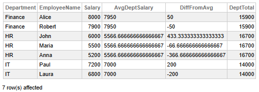Fig 1 - Department Salary Analytics

The data above help us conclude the following key findings:

Finance department salaries are closely aligned with the average: Alice earns slightly above (+50), Robert slightly below (−50), indicating balanced compensation.
HR department reveals a significant salary disparity: John earns well above the average (+433.33), while Anna earns far below (−366.67), suggesting potential inequity or role-based differentiation.
Maria’s salary in HR is near the average (−66.67), acting as a midpoint between extremes.
The IT department exhibits symmetrical deviation: Paul earns +200 above the average, Laura −200 below, implying a clear salary tiering.
Department totals show that HR has the highest aggregate salary (16,700), followed by Finance (15,900) and IT (14,000), possibly reflecting headcount or budget allocation.
Average salary per department: Finance (7,950), HR (5,566.67), IT (7,000), with HR notably lower, pointing out different job levels or market rates.

👉 Why it is useful: You can compare individuals to their group (department average) without collapsing the dataset. It is ideal for identifying outliers or salary imbalances.

Example 2 — Clinic Workload Analysis

Let’s assess how each physician’s daily workload compares to their department’s total.

CREATE TABLE Appointments (  
    Department VARCHAR(50),  
    Physician VARCHAR(50),  
    DailyAppointments INTEGER  
)

INSERT INTO Appointments  
SELECT 'Cardiology','Dr. Smith',18 UNION ALL
SELECT 'Cardiology','Dr. Lee',22 UNION ALL
SELECT 'Cardiology','Dr. Adams',16 UNION ALL
SELECT 'Pediatrics','Dr. Young',25 UNION ALL
SELECT 'Pediatrics','Dr. Patel',30 UNION ALL
SELECT 'Neurology','Dr. Miller',15

We need to do the next:

Calculate the total daily appointments for each Department using a window function (SUM() OVER (PARTITION BY Department)).
Determine the percentage of the department's total appointments contributed by each Physician (WorkloadPercentage).
Display all individual physician/appointment rows alongside these computed department totals and percentages.
Order the final result set by Department and then by DailyAppointments (highest first).

SELECT  
    Department,  
    Physician,  
    DailyAppointments,  
    SUM(DailyAppointments) OVER (PARTITION BY Department) AS DeptTotalAppointments,  
    ROUND(  
        100.0 * DailyAppointments /
        SUM(DailyAppointments) OVER (PARTITION BY Department), 2  
    ) AS WorkloadPercentage  
FROM Appointments  
ORDER BY Department, DailyAppointments DESC

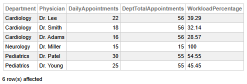Fig 2 - Clinic Workload Analysis

This data allows us to identify the following key findings:

The cardiology department exhibits a balanced workload distribution: Dr. Lee handles the largest share (39.29%), followed by Dr. Smith (32.14%) and Dr. Adams (28.57%), indicating no extreme disparities.
Neurology is a single-physician department: Dr. Miller carries 100% of the workload, suggesting full responsibility and potential overreliance on a single provider.
Pediatrics has a moderate imbalance: Dr. Patel manages a larger portion (54.55%) compared to Dr. Young (45.45%), pointing out a slightly uneven patient load.
Total appointments per department: Cardiology (56), Pediatrics (55), Neurology (15), with Cardiology and Pediatrics having similar volumes whereas Neurology displays a significantly lower one.
Highest individual workload: Dr. Patel (30 appointments), followed by Dr. Lee (22), implying potential scheduling or capacity considerations.

👉 Why it is useful: Understanding how much each doctor contributes to the department workload is ideal for balancing resources.

2. Ranking and Distribution Functions

Overview

These functions assign rankings or distributions to rows within a partition.
Unlike aggregates, they provide relative position or percentile context.

Functions:

ROW_NUMBER() — a unique sequential integer assigned to each row.
RANK() — appoints ranks with gaps for ties.
DENSE_RANK() — determines ranks without gaps.
NTILE(num_groups) — divides rows into roughly equal groups and returns the group number.
PERCENT_RANK() — a fractional rank, calculated as (rank-1)/(rows-1).
CUME_DIST() — cumulative distribution, calculated as rows with value ≤ current row value / total rows.

Example 1 — Hospital Department Satisfaction Ranking

Let’s evaluate how the average satisfaction score of each hospital department compares across the organization.

CREATE TABLE DepartmentSatisfaction (  
    Department VARCHAR(50),  
    Month VARCHAR(10),
    AvgSatisfaction DECIMAL(5,2)  
)

INSERT INTO DepartmentSatisfaction  
SELECT 'Cardiology','Jan',4.6 UNION ALL
SELECT 'Cardiology','Feb',4.8 UNION ALL
SELECT 'Cardiology','Mar',4.9 UNION ALL
SELECT 'Neurology','Jan',4.7 UNION ALL
SELECT 'Neurology','Feb',4.7 UNION ALL
SELECT 'Neurology','Mar',4.9 UNION ALL
SELECT 'Pediatrics','Jan',4.9 UNION ALL
SELECT 'Pediatrics','Feb',4.8 UNION ALL
SELECT 'Pediatrics','Mar',4.9 UNION ALL
SELECT 'Oncology','Jan',4.5 UNION ALL
SELECT 'Oncology','Feb',4.7 UNION ALL
SELECT 'Oncology','Mar',4.7

We should do the following:

Calculate the average satisfaction score for each Department using AVG() OVER within a grouped query.
Apply three ranking functions to compare behavior:
- ROW_NUMBER() for strict ordering.
- RANK() to show gaps in ranking when ties occur.
- DENSE_RANK() to group tied departments without gaps.
Order the final result by average satisfaction (highest first).

SELECT  
    Department,  
    ROUND(AVG(AvgSatisfaction),2) AS DeptAvgSatisfaction,
    ROW_NUMBER() OVER (ORDER BY AVG(AvgSatisfaction) DESC) AS AvgSatisfactionRowNumber,
    RANK() OVER (ORDER BY AVG(AvgSatisfaction) DESC) AS AvgSatisfactionRankValue,
    DENSE_RANK() OVER (ORDER BY AVG(AvgSatisfaction) DESC) AS AvgSatisfactionDenseRankValue
FROM DepartmentSatisfaction  
GROUP BY Department
ORDER BY DeptAvgSatisfaction DESC

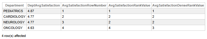Fig 3 - Hospital Department Satisfaction Ranking

This data enables us to make the following key findings:

Pediatrics leads in satisfaction with the highest average score (4.87), earning the top rank across all metrics.
Cardiology and Neurology share the same average satisfaction (4.77), resulting in a tie for rank 2 in both standard and dense ranking systems.
Oncology has the lowest satisfaction score (4.63), placing it last in the row number and rank value, but third in the dense rank due to the tie above.
Satisfaction scores are tightly clustered, with a spread of only 0.24 between the highest and lowest, indicating generally high satisfaction across departments.

👉 Why it is useful: Comparing department performance with flexible ranking views (ROW_NUMBER() for unique order, RANK() for competitive gaps, and DENSE_RANK() for grouped ties) is ideal for performance dashboards or leaderboards.

Example 2 — Product Performance Ranking

Let’s evaluate how each product’s sales performance compares within its category using percentile-based ranking functions.

CREATE TABLE Sales (  
    Category VARCHAR(50),  
    Product VARCHAR(50),  
    Sales INTEGER  
)

INSERT INTO Sales  
SELECT 'Electronics','Phone',1200 UNION ALL
SELECT 'Electronics','Tablet',900 UNION ALL
SELECT 'Electronics','TV',1500 UNION ALL
SELECT 'Electronics','Camera',1100 UNION ALL
SELECT 'Furniture','Chair',400 UNION ALL
SELECT 'Furniture','Table',700 UNION ALL
SELECT 'Furniture','Desk',650

We need to:

Divide products into quartiles within each category using NTILE(4) OVER (PARTITION BY Category ORDER BY Sales DESC).
Calculate percentile rank of each product using PERCENT_RANK() OVER (PARTITION BY Category ORDER BY Sales).
Compute cumulative distribution using CUME_DIST() OVER (PARTITION BY Category ORDER BY Sales).
Order the final result by Category and then by Sales (highest first).

SELECT  
    Category,  
    Product,  
    Sales,  
    NTILE(4) OVER (PARTITION BY Category ORDER BY Sales DESC) AS Quartile,  
    PERCENT_RANK() OVER (PARTITION BY Category ORDER BY Sales) AS PercentRank,
    CUME_DIST() OVER (PARTITION BY Category ORDER BY Sales) AS CumulativeDist
FROM Sales  
ORDER BY Category, Sales DESC

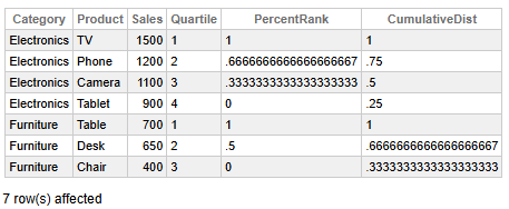Fig 4 - Product Performance Ranking

This data helps us conclude the next key findings:

TV and Table are the top-selling products in their respective categories, both ranked in Quartile 1 with perfect PercentRank and CumulativeDist scores of 1.
Electronics show a clear descending sales pattern compared to the TV and the Table, with each product occupying a lower quartile and percentile rank, indicating a well-stratified performance distribution.
Furniture sales also decline from the Table to the Chair. However, the drop is steeper and less evenly distributed, suggesting a more concentrated demand for top-tier items.
Tablet and Chair are the lowest performers in their respective categories, both with a PercentRank of 0 and a CumulativeDist below 0.35, indicating a minimal relative sales impact.
Phone and Desk occupy mid-tier positions in their categories, with PercentRanks between 0.5 and 0.67, reflecting moderate performance.

👉 Why it is useful: Identifying top-performing products and categorizing them by percentile for dashboards is ideal for sales strategy and inventory planning.

Example 3 — Hospital Performance Quartiles

Let’s categorize hospital departments based on their monthly patient volume using quartiles and cumulative distribution.

CREATE TABLE DepartmentMetrics (  
    Department VARCHAR(50),  
    PatientCount INTEGER  
)

INSERT INTO DepartmentMetrics  
SELECT 'Cardiology',1200 UNION ALL
SELECT 'Pediatrics',950 UNION ALL
SELECT 'Neurology',800 UNION ALL
SELECT 'Orthopedics',700 UNION ALL
SELECT 'Dermatology',500 UNION ALL
SELECT 'Oncology',600

We should do the next:

Use NTILE(4) to divide departments into quartiles based on PatientCount.
Apply CUME_DIST() to compute the cumulative distribution of departments by patient volume.
Order the final result by PatientCount (ascending) to visualize performance tiers.

SELECT  
    Department,  
    PatientCount,  
    NTILE(4) OVER (ORDER BY PatientCount) AS Quartile,  
    CUME_DIST() OVER (ORDER BY PatientCount) AS CumulativeDistribution
FROM DepartmentMetrics  
ORDER BY PatientCount

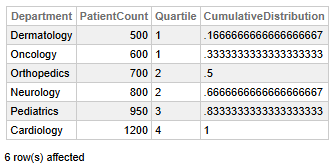Fig 5 - Hospital Performance Quartiles

This data permits us to discover the following key findings:

Cardiology has the highest patient count (1,200), placing it in Quartile 4 with a full cumulative distribution (1), indicating that it serves the largest share of patients.
Dermatology and Oncology fall into Quartile 1 with lower patient counts (500 and 600), representing the bottom third of departmental volumes.
Orthopedics and Neurology are mid-range in Quartile 2, with patient counts of 700 and 800, respectively, showing moderate service levels.
Pediatrics ranks in Quartile 3 with 950 patients, suggesting the above-average volume, however, not the highest.

👉 Why it is useful: Quickly classifying departments into performance bands for hospital management is ideal for resource allocation and strategic planning.

3. Final Thoughts

Stay tuned for the final installment of this Window Functions introduction, where we will explore another powerful group of functions. You will also get performance optimization tips and a practical guide to help you decide when to use and when to avoid window functions.

This article was written with the help of AI tools to clarify concepts and improve readability.