Python JDBC connection into IRIS database - a quick note
Keywords: Python, JDBC, SQL, IRIS, Jupyter Notebook, Pandas, Numpy, and Machine Learning
1. Purpose
This is another 5-minute simple note on invoking the IRIS JDBC driver via Python 3 within i.e. a Jupyter Notebook, to read from and write data into an IRIS database instance via SQL syntax, for demo purpose.
Last year I touched on a brief note on Python binding into a Cache database (section 4.7) instance. Now it might be time to recap some options and discussions on using Python to hook into an IRIS database, to read its data into a Pandas dataframe and a NumPy array for normal analysis, then to write some pre-processed or normalised data back into IRIS ready for further ML/DL pipelines.
Immediately there would be a few quick options popping out on top of the head:
- ODBC: How about PyODBC for Python 3 and native SQL?
- JDBC: How about JayDeBeApi for Pyhton 3 and native SQL?
- Spark: How about the PySpark and SQL?
- Python Native API for IRIS: beyond the previous Python Binding for Cache?
- IPtyhon Magic SQL %%sql? Could it work with IRIS yet?
Any other options being missed here? I am interested in trying them too.
2. Scope
Shall we just start with a normal JDBC approach? We will recap on ODBC, Spark and Python Native API in next brief note.
In Scope:
The following common components are touched in this quick demo:
- Anaconda
- Jupyter Notebook
- Python 3
- JayDeBeApi
- JPyPe
- Pandas
- NumPy
- An IRIS 2019.x instance
Out of Scope:
The following will NOT be touched in this quick note - they are important, and can be addressed separately with specific site solutions, deployments and services:
- Security end-2-end.
- Non-functional performance etc.
- Trouble-shooting and Support.
- Licensing.
3. Demo
3.1 Run an IRIS instance:
I simply ran an IRIS 2019.4 container as a "remote" database server. You can use any IRIS instance to which you have the right authorised access.
zhongli@UKM5530ZHONGLI MINGW64 /c/Program Files/Docker Toolbox
$ docker ps
CONTAINER ID IMAGE COMMAND CREATED STATUS PORTS NAMES
d86be69a03ab quickml-demo "/iris-main" 3 days ago Up 3 days (healthy) 0.0.0.0:9091->51773/tcp, 0.0.0.0:9092->52773/tcp quickml
3.2 Anaconda and Jupyter Notebook:
We will reuse the same setup approach as described here for Anaconda (section 4.1) and here for Jupyter Notebook (section 4) in a laptop. Python 3.x is installed along with this step.
3.3 Install JayDeBeApi and JPyPe:
!conda install --yes -c conda-forge jaydebeapiJayDeBeApi uses JPype 0.7 at the time of writing (Jan 2020) - it doesn't work due to a known bug, so had to be downgraded to 0.6.3
!conda install --yes -c conda-forge JPype1=0.6.3 --force-reinstall3.4 Connect into IRIS database via JDBC
There is an official JDBC into IRIS documentation here.
For Python SQL executions over JDBC , I used the following codes as an example. It connects into a data table called "DataMining.IrisDataset" within "USER" namespace of this IRIS instance.
### 1. Set environment variables, if necessary
#import os
#os.environ['JAVA_HOME']='C:\Progra~1\Java\jdk1.8.0_241'
#os.environ['CLASSPATH'] = 'C:\interSystems\IRIS20194\dev\java\lib\JDK18\intersystems-jdbc-3.0.0.jar'
#os.environ['HADOOP_HOME']='C:\hadoop\bin'  #winutil binary must be in Hadoop's Home
### 2. Get jdbc connection and cursor
import jaydebeapi
url = "jdbc:IRIS://192.168.99.101:9091/USER"
driver = 'com.intersystems.jdbc.IRISDriver'
user = "SUPERUSER"
password = "SYS"
#libx = "C:/InterSystems/IRIS20194/dev/java/lib/JDK18"
jarfile = "C:/InterSystems/IRIS20194/dev/java/lib/JDK18/intersystems-jdbc-3.0.0.jar"conn = jaydebeapi.connect(driver, url, [user, password], jarfile)
curs = conn.cursor()### 3. specify the source data table
dataTable = 'DataMining.IrisDataset'### 4. Get the result and display
curs.execute("select TOP 20 * from %s" % dataTable)
result = curs.fetchall()
print("Total records: " + str(len(result)))
for i in range(len(result)):
print(result[i])### 5. CLose and clean - I keep them open for next accesses.
#curs.close()
#conn.close()
Total records: 150
(1, 1.4, 0.2, 5.1, 3.5, 'Iris-setosa')
(2, 1.4, 0.2, 4.9, 3.0, 'Iris-setosa')
(3, 1.3, 0.2, 4.7, 3.2, 'Iris-setosa')
... ...
(49, 1.5, 0.2, 5.3, 3.7, 'Iris-setosa')
(50, 1.4, 0.2, 5.0, 3.3, 'Iris-setosa')
(51, 4.7, 1.4, 7.0, 3.2, 'Iris-versicolor')
... ...
(145, 5.7, 2.5, 6.7, 3.3, 'Iris-virginica')
... ...
(148, 5.2, 2.0, 6.5, 3.0, 'Iris-virginica')
(149, 5.4, 2.3, 6.2, 3.4, 'Iris-virginica')
(150, 5.1, 1.8, 5.9, 3.0, 'Iris-virginica')
Now we tested that Python on JDBC was working. The following is just a bit of routine data analysis and preprocessing for usual ML pipelines that we might touch on again and again for later demos and comparisons hence is attached for conveniences.
3.5 Convert SQL results to Pandas DataFrame then NumPy Array
Install Pandas and NumPy packages via Conda if they are not installed yet, similar to section 3.3 above.
Then ran the following as an example:
import pandas as pd
sqlData = "SELECT * from DataMining.IrisDataset"
df= pd.io.sql.read_sql(sqlData, conn)
df = df.drop('ID', 1)
df = df[['SepalLength', 'SepalWidth', 'PetalLength', 'PetalWidth', 'Species']]
df.replace('Iris-setosa', 0, inplace=True)
df.replace('Iris-versicolor', 1, inplace=True)
df.replace('Iris-virginica', 2, inplace=True)
arrayN = df.to_numpy()
#curs.close()
#conn.close()
Let's have a routine peek into current data:
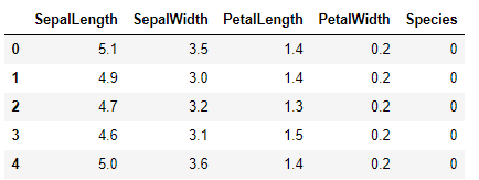

Now we got a DataFrame, and a normalised NumPy array from a source data table to our disposal.
Certainly, here we can try various routine analysis that a ML person would start with, as below, in Python to replace R as the link here?

Data source is quoted from here
3.6 Split data and write back into IRIS database via SQL:
Certainly we can split the data into a Training and a Validation or Test set, as usual, then write them back into temporary database tables, for some exciting on-coming ML features of IRIS:
from matplotlib import pyplot
from sklearn.model_selection import train_test_split
X = arrayN[:,0:4]
y = arrayN[:,4]
X_train, X_validation, Y_train, Y_validation = train_test_split(X, y, test_size=0.20, random_state=1, shuffle=True)
labels1 = np.reshape(Y_train,(120,1))
train = np.concatenate([X_train, labels1],axis=-1)
lTest1 = np.reshape(Y_validation,(30,1))
test = np.concatenate([X_validation, lTest1],axis=-1)
dfTrain = pd.DataFrame({'SepalLength':train[:, 0], 'SepalWidth':train[:, 1], 'PetalLength':train[:, 2], 'PetalWidth':train[:, 3], 'Species':train[:, 4]})
dfTrain['Species'].replace(0, 'Iris-setosa', inplace=True)
dfTrain['Species'].replace(1, 'Iris-versicolor', inplace=True)
dfTrain['Species'].replace(2, 'Iris-virginica', inplace=True)
dfTest = pd.DataFrame({'SepalLength':test[:, 0], 'SepalWidth':test[:, 1], 'PetalLength':test[:, 2], 'PetalWidth':test[:, 3], 'Species':test[:, 4]})
dfTest['Species'].replace(0, 'Iris-setosa', inplace=True)
dfTest['Species'].replace(1, 'Iris-versicolor', inplace=True)
dfTest['Species'].replace(2, 'Iris-virginica', inplace=True)
#dataTable = 'DataMining.IrisDataset'
dtTrain = 'TRAIN02'
dtTest = "TEST02"
curs.execute("Create Table %s (%s DOUBLE, %s DOUBLE, %s DOUBLE, %s DOUBLE, %s VARCHAR(100))" % (dtTrain, dfTrain.columns[0], dfTrain.columns[1], dfTrain.columns[2], dfTrain.columns[3], dfTrain.columns[4]))
curs.execute("Create Table %s (%s DOUBLE, %s DOUBLE, %s DOUBLE, %s DOUBLE, %s VARCHAR(100))" % (dtTest, dfTest.columns[0], dfTest.columns[1], dfTest.columns[2], dfTest.columns[3], dfTest.columns[4]))
curs.fast_executemany = True
curs.executemany( "INSERT INTO %s (SepalLength, SepalWidth, PetalLength, PetalWidth, Species) VALUES (?, ?, ?, ? ,?)" % dtTrain,
list(dfTrain.itertuples(index=False, name=None)) )
curs.executemany( "INSERT INTO %s (SepalLength, SepalWidth, PetalLength, PetalWidth, Species) VALUES (?, ?, ?, ? ,?)" % dtTest,
list(dfTest.itertuples(index=False, name=None)) )
#curs.close()
#conn.close()
Now if we switch to IRIS Management Console, or Terminal SQL Console, we should see 2 temp tables created: TRAIN02 with 120 rows and TEST02 with 30 rows.
I will have to stop here, as it's supposedly be a very brief quick note.
4. Caveats
- The content above may be changed or refined.
5. Next
We will simply replace section 3.3 and 3.4 with PyODBC, PySPark and Python Native API for IRIS, unless anyone wouldn't mind helping contribute a quick note as well - I will appreciate too.
Comments
💡 This article is considered as InterSystems Data Platform Best Practice.