Explainability and Visibility into Covid-19 X-Ray Classifiers by Deep Learning

Keywords: Deep Learning, Grad-CAM, X-Ray, Covid-19, HealthShare, IRIS

Purpose

Over the Easter Weekend I touched on some deep learning classifier for Covid-19 Lungs.  The demo result seems fine, seemingly matching some academic research publications around that time on this topic. But is it really "fine "? 

Recently I happened to listen to an online lunch webinar on "Explainability  in Machine Learning", and Don talked about this classification result at the end of his talk:

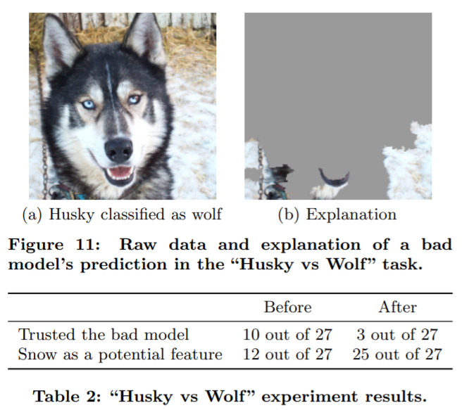
The above figure is also presented in this research paper: “Why Should I Trust You?” Explaining the Predictions of Any Classifier .   We can see that the classifier was actually trained to take the background pixels,  e.g. snow etc wild environment, as main inputs to classify whether it's a pet dog or a wild wolf. 

That  invokes my old interests, and surely stirs up a bit curiosity for now:

• How could we "look into" these Covid-19 classifiers, normally presented as "black boxes" , to see what pixels actually contributed to a "Covid-19 Lung" result?
• What's the simplest approach in its simplest form or simplest tool that we could leverage in this case? 

This is another 10-minute note along the journey. In the end I might touch on why it's related to our on-coming and exciting new IRIS and HealthShare features too.

Scope

Fortunately over the past few years, there are convenient tools coming up for various CNN derived classifiers:

• CAM (Class Activation Map) :  its applications are well explained here and here.  
• Grad-CAM (Gradient-weighted Class  Activation) : which is a more generic version of CAM, which enables us to look into any CNN layers within the whole model.

We will use Grad-CAM to do a quick demo into our previous Covid-19 lung classifier in the previous post.

"Tensorflow 2.2.0rc + Jupyter" Docker is used on an AWS Ubuntu 16.04 server with Nvidia T4 GPU.   Tensorflow 2 provides a simple "Gradient-Tape" implementation. 

Here is my quick note to start it on the Ubuntu server:  

docker run -itd --runtime=nvidia  -v /zhong/tf/:/tf  -p 8896:8888 -p 6026:6006 --name tf-gpu2 tensorflow/tensorflow:2.2.0rc2-gpu-py3-jupyter

Method

You can safely ignore a bit math quoted here from above Grad-CAM research publications.

It's quoted here just for our continuous cross-checking  of the original proposal (in page 4 & 5) against Python code being used later, hoping to provide better transparency on the result too.

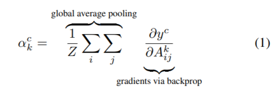
(1): To obtain the class discriminative localization map of width u and height v for any class c, we first compute the gradient of the score for the class c, yc (before the softmax) with respect to feature maps Ak of a convolutional layer. These gradients flowing back are global average-pooled to obtain the neuron importance weights ak for the target class.

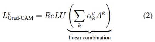
(2): After calculating ak for the target class c, we perform a weighted combination of activation maps and follow it by ReLU.  This results in a coarse heatmap of the same size as that of the convolutional feature maps.  

Test

Now let's try the bit simplest coding that we could find so far:

1. Import the packages

import tensorflow as tf;
print(tf.__version__)

2.2.0-rc2

import tensorflow as tf
import tensorflow.keras.backend as K
from tensorflow.keras.applications.inception_v3 import InceptionV3
from tensorflow.keras.preprocessing import image
from tensorflow.keras.applications.inception_v3 import preprocess_input, decode_predictions
import numpy as np
import os
import imutils
import matplotlib.pyplot as plt
import cv2

2. Load our previously trained and saved model

new_model = tf.keras.models.load_model('saved_model/inceptionV3')
new_model.summary()

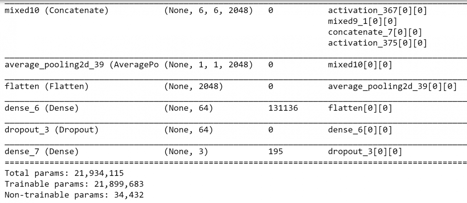
We can see that the last CNN layer of 4D in our model is called "mixed10" before the final global average pooling. 

3. Compute  a Grad-CAM heatmap  

There is a simple version of the heatmap as below, implementing above Grad-CAM equation (1) & (2).  It is explained in this post. 

with tf.GradientTape() as tape:
  last_conv_layer = model.get_layer('mixed10') 
  iterate = tf.keras.models.Model([model.inputs], [model.output, last_conv_layer.output])
  model_out, last_conv_layer = iterate(testX)
  class_out = model_out[:, np.argmax(model_out[0])]
  grads = tape.gradient(class_out, last_conv_layer)
  pooled_grads = K.mean(grads, axis=(0, 1, 2))
  heatmap = tf.reduce_mean(tf.multiply(pooled_grads, last_conv_layer), axis=-1)

 It will generate a heatmap numpy array of (27, 6, 6) in our case. Then we can re-size it to our original X-Ray image size  and overlay it on top of the X-Ray image - that's it.

However, in this case, we will use a slightly more verbose version that is explained really well in this post  too. It composed a function with the Grad-CAM heatmap already resized as that of original X-Ray:

# import the necessary packages
from tensorflow.keras.models import Model
import tensorflow as tf
import numpy as np
import cv2

class GradCAM:
    def __init__(self, model, classIdx, layerName=None):
        self.model = model
        self.classIdx = classIdx
        self.layerName = layerName
        if self.layerName is None:
            self.layerName = self.find_target_layer()

    def find_target_layer(self):
        for layer in reversed(self.model.layers):
            # check to see if the layer has a 4D output
            if len(layer.output_shape) == 4:
                return layer.name
        raise ValueError("Could not find 4D layer. Cannot apply GradCAM.")

    def compute_heatmap(self, image, eps=1e-8):
        gradModel = Model(
            inputs=[self.model.inputs],
            outputs=[self.model.get_layer(self.layerName).output,
                self.model.output])
        # record operations for automatic differentiation
        with tf.GradientTape() as tape:
            inputs = tf.cast(image, tf.float32)
            (convOutputs, predictions) = gradModel(inputs)
            loss = predictions[:, self.classIdx]
        # use automatic differentiation to compute the gradients
        grads = tape.gradient(loss, convOutputs)
        # compute the guided gradients
        castConvOutputs = tf.cast(convOutputs > 0, "float32")
        castGrads = tf.cast(grads > 0, "float32")
        guidedGrads = castConvOutputs * castGrads * grads
        convOutputs = convOutputs[0]
        guidedGrads = guidedGrads[0]
        weights = tf.reduce_mean(guidedGrads, axis=(0, 1))
        cam = tf.reduce_sum(tf.multiply(weights, convOutputs), axis=-1)

        # resize the heatmap to oringnal X-Ray image size
        (w, h) = (image.shape[2], image.shape[1])
        heatmap = cv2.resize(cam.numpy(), (w, h))

        # normalize the heatmap
        numer = heatmap - np.min(heatmap)
        denom = (heatmap.max() - heatmap.min()) + eps
        heatmap = numer / denom
        heatmap = (heatmap * 255).astype("uint8")

        # return the resulting heatmap to the calling function
        return heatmap

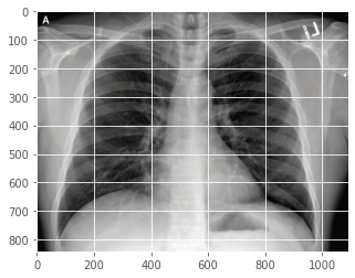
4. Load a Covid-19 lung X-Ray

Now we load a test X-Ray that was never used in model training and validation process. (It was also uploaded into the previous post)

filename = './test/nejmoa2001191_f1-PA.jpeg'
orignal = cv2.imread(filename)
plt.imshow(orignal)
plt.show()

Then resize to 256 x 256, and normalise it into a numpy array "dataXG" of pixel value between 0.0 and 1.0.

orig = cv2.cvtColor(orignal, cv2.COLOR_BGR2RGB)
resized = cv2.resize(orig, (256, 256))
dataXG = np.array(resized) / 255.0
dataXG = np.expand_dims(dataXG, axis=0)

5. Conduct a quick classification 

 Now we can call the newly loaded model above to do a quick prediction:

preds = new_model.predict(dataXG)
i = np.argmax(preds[0])
print(i, preds)

0     [[0.9171522  0.06534185 0.01750595]]

So it is classified as type 0 -    a Covid-19 lung with a probability of 0.9171522.

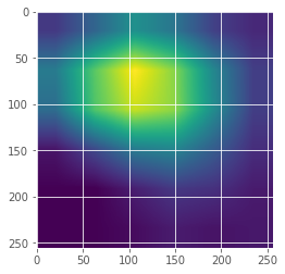
6. Compute the Grad-CAM Heatmap

# Compute the heatmap based on step 3
cam = GradCAM(model=new_model, classIdx=i, layerName='mixed10') # find the last 4d shape "mixed10" in this case
heatmap = cam.compute_heatmap(dataXG)

#show the calculated heatmap
plt.imshow(heatmap)
plt.show()

7. Display the heatmap onto original X-ray

# Old fashioned way to overlay a transparent heatmap onto original image, the same as above
heatmapY = cv2.resize(heatmap, (orig.shape[1], orig.shape[0]))
heatmapY = cv2.applyColorMap(heatmapY, cv2.COLORMAP_HOT)  # COLORMAP_JET, COLORMAP_VIRIDIS, COLORMAP_HOT
imageY = cv2.addWeighted(heatmapY, 0.5, orignal, 1.0, 0)
print(heatmapY.shape, orig.shape)

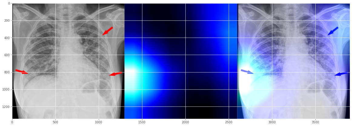
# draw the orignal x-ray, the heatmap, and the overlay together
output = np.hstack([orig, heatmapY, imageY])
fig, ax = plt.subplots(figsize=(20, 18))
ax.imshow(np.random.rand(1, 99), interpolation='nearest')
plt.imshow(output)
plt.show()

(842, 1090, 3) (842, 1090, 3)

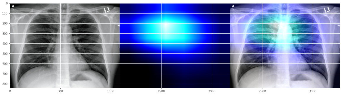It seems to indicate that our Covid-19 demo classifier "believes" that the patient got a bit "opacification "issue around the "right para tracheal stripe"? I don't really know unless I check with the a real radiologist.

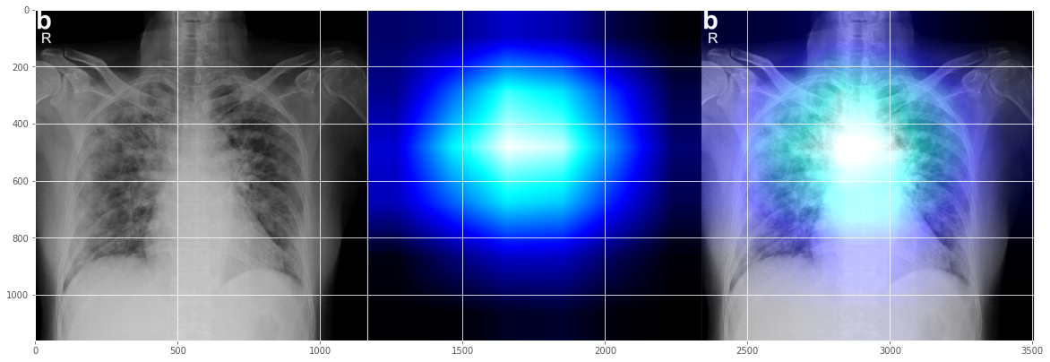
OK, let's try a few more test images submitted from some real-world cases into the github repository:

filename = './test/1-s2.0-S0929664620300449-gr2_lrg-b.jpg'

0    [[9.9799889e-01 3.8319459e-04 1.6178709e-03]]

This seems a reasonable-looking Covid-19 interpretation as well, indicating issues happening more on left heart line area?

Let's try another random test x-ray:

filename = '../Covid_M/all/test/covid/radiol.2020200490.fig3.jpeg'

0      [[0.9317619  0.0169084  0.05132957]]

Surprisingly, this doesn't look exactly right, but look it again it seems not too off-mark either, right?  It shows two issue areas - the major problem on the left side, and some issue on the right side, somewhat aligned with the human radiologist's markup? (While hoping it's not being trained on the human markers - that's another level of explainability issue).

OK, I will have to stop here, since not sure too many people would be interested in reading X-Ray anyway in this 10-minute quite note.

Why?

I personally deeply appreciate the importance of "Explainability" and "Interpretability" and any technical approaches towards them.  Any slight attempts into this dimension are worthy of the efforts, no matter how tiny they are. Eventually "Data Fairness", "Data Justice" , and "Data Trust" will be built on its Process Transparency in digital economies.  Also, it starts to become available now.     25 years back when I was young and doing my PhD thesis for the whole summer of 1995, I didn't even hope to get slight sense out of the so called "Neural Networks" largely used as black boxes. At that time AI was more about "Expert System" as logical reasoning machine; and "Neural Networks" were called "Neural Networks" - "Deep Learning" had not been born yet. Now we have more and more researches and tools, right at the finger tip of today's AI developers. 

Last but not the least, specific to this demo, one thing I could appreciate of such tools is it doesn't even need a pixel-grade labeling to start with -  it attempted to automatically generate pulmonary lesion area for you, kind of semi-automatic labeling. It means something in real works.   I do remember last year a radiologist friend of mine was helping me generate a few pixel grade labels for U-Net training again and again for some bone fracture data - that exercise did hurt our eyes. 

Next

I wandered a bit off by now. Medical Imaging is a relatively mature direction in AI fields, thanks to the fast advancement of Deep Learning in the past 10+ years. It's worthy of some good time. However, next I wish we could try more on the NLP fronts, if we could have a bit time ever.   

Acknowledgement

All sources have been inserted into the above texts wherever it is needed. I will put in more references if needed too.  

Disclaimer: 

Again, the above is supposed to be a quick note in case it's just gone after another few weeks if I don't record it for now. All are personal views as a "Developer". The content and texts may be revised anytime as needed. The above is more about demonstrating the technology ideas and approaches than clinical interpretations, for which specialist radiologist will be needed to set up golden rules on a good quantity and quality of data.