Bridge AI/ML with your Adaptive Analytics solution

In today's data landscape, businesses encounter a number of different challenges. One of them is to do analytics on top of unified and harmonized data layer available to all the consumers. A layer that can deliver the same answers to the same questions irrelative to the dialect or tool being used.
InterSystems IRIS Data Platform answers that with and add-on of Adaptive Analytics that can deliver this unified semantic layer. There are a lot of articles in DevCommunity about using it via BI tools. This article will cover the part of how to consume it with AI and also how to put some insights back.
Let's go step by step...

What is Adaptive Analytics?

You can easily find some definition in developer community website
In a few words, it can deliver data in structured and harmonized form to various tools of your choice for further consumption and analysis. It delivers the same data structures to various BI tools. But... it can also deliver same data structures to your AI/ML tools!

Adaptive Analytics has and additional component called AI-Link that builds this bridge from AI to BI.

What exactly is AI-Link ?

It is a Python component that is designed to enable programmatic interaction with the semantic layer for the purposes of streamlining key stages of the machine learning (ML) workflow (for example, feature engineering).

With AI-Link you can:
* programmatically access features of your analytical data model;
* make queries, explore dimensions and measures;
* feed ML pipelines;
... and deliver results back to your semantic layer to be consumed again by others (e.g. through Tableau or Excel).

As this is a Python library, it can be used in any Python environment. Including Notebooks.
And in this article I'll give a simple example of reaching Adaptive Analytics solution from Jupyter Notebook with the help of AI-Link.

Here is git repository which will have the complete Notebook as example: https://github.com/v23ent/aa-hands-on

Pre-requisites

Further steps assume that you have the following pre-requisites completed:
1. Adaptive Analytics solution up and running (with IRIS Data Platform as Data Warehouse)
2. Jupyter Notebook up and running
3. Connection between 1. and 2. can be established

Step 1: Setup

First, let's install needed components in our environment. That will download a few packages needed for further steps to work.
'atscale' - this is our main package to connect
'prophet' - package that we'll need to do predictions

pip install atscale prophet

Then we'll need to import key classes representing some key concepts of our semantic layer.
Client - class that we'll use to establich a connection to Adaptive Analytics;
Project - class to represent projects inside Adaptive Analytics;
DataModel - class that will represent our virtual cube;

from atscale.client import Client
from atscale.data_model import DataModel
from atscale.project import Project
from prophet import Prophet
import pandas as pd 

Step 2: Connection

Now we should be all set to establish a connection to our source of data.

client = Client(server='http://adaptive.analytics.server', username='sample')
client.connect()

Go ahead and specify connection details of your Adaptive Analytics instance. Once you're asked for the organization respond in the dialog box and then please enter your password from the AtScale instance.

With established connection you'll then need to select your project from the list of projects published on the server. You'll get the list of projects as an interactive prompt and the answer should be the integer ID of the project. And then data model is selected automatically if it's the only one.

project = client.select_project()   
data_model = project.select_data_model()

Step 3: Explore your dataset

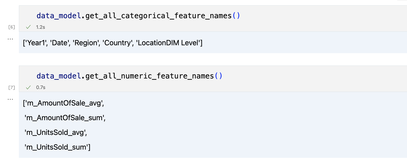
There are a number of methods prepared by AtScale in AI-Link component library. They allow to explore data catalog that you have, query data, and even ingest some data back. AtScale documentation has extensive API reference describing everything that is available.
Let's first see what is our dataset by calling few methods of data_model:

data_model.get_features()
data_model.get_all_categorical_feature_names()
data_model.get_all_numeric_feature_names()

The output should look something like this

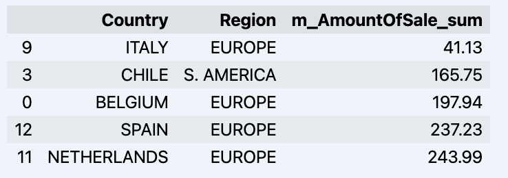
Once we've looked around a bit, we can query the actual data we're interested in using 'get_data' method. It will return back a pandas DataFrame containing the query results.

df = data_model.get_data(feature_list = ['Country','Region','m_AmountOfSale_sum'])
df = df.sort_values(by='m_AmountOfSale_sum')
df.head()

Which will show your datadrame:

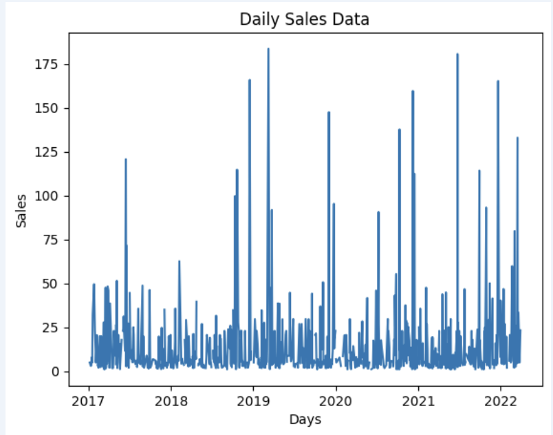
Let's prepare some dataset and quickly show it on the graph

import matplotlib.pyplot as plt

# We're taking sales for each date
dataframe = data_model.get_data(feature_list = ['Date','m_AmountOfSale_sum'])

# Create a line chart
plt.plot(dataframe['Date'], dataframe['m_AmountOfSale_sum'])

# Add labels and a title
plt.xlabel('Days')
plt.ylabel('Sales')
plt.title('Daily Sales Data')

# Display the chart
plt.show()

Output:

Step 4: Prediction

The next step would be to actually get some value out of AI-Link bridge - let's do some simple prediction!

# Load the historical data to train the model
data_train = data_model.get_data(
    feature_list = ['Date','m_AmountOfSale_sum'],
    filter_less = {'Date':'2021-01-01'}
    )
data_test = data_model.get_data(
    feature_list = ['Date','m_AmountOfSale_sum'],
    filter_greater = {'Date':'2021-01-01'}
    )

We get 2 different datasets here: to train our model and to test it.

# For the tool we've chosen to do the prediction 'Prophet', we'll need to specify 2 columns: 'ds' and 'y'
data_train['ds'] = pd.to_datetime(data_train['Date'])
data_train.rename(columns={'m_AmountOfSale_sum': 'y'}, inplace=True)
data_test['ds'] = pd.to_datetime(data_test['Date'])
data_test.rename(columns={'m_AmountOfSale_sum': 'y'}, inplace=True)

# Initialize and fit the Prophet model
model = Prophet()
model.fit(data_train)

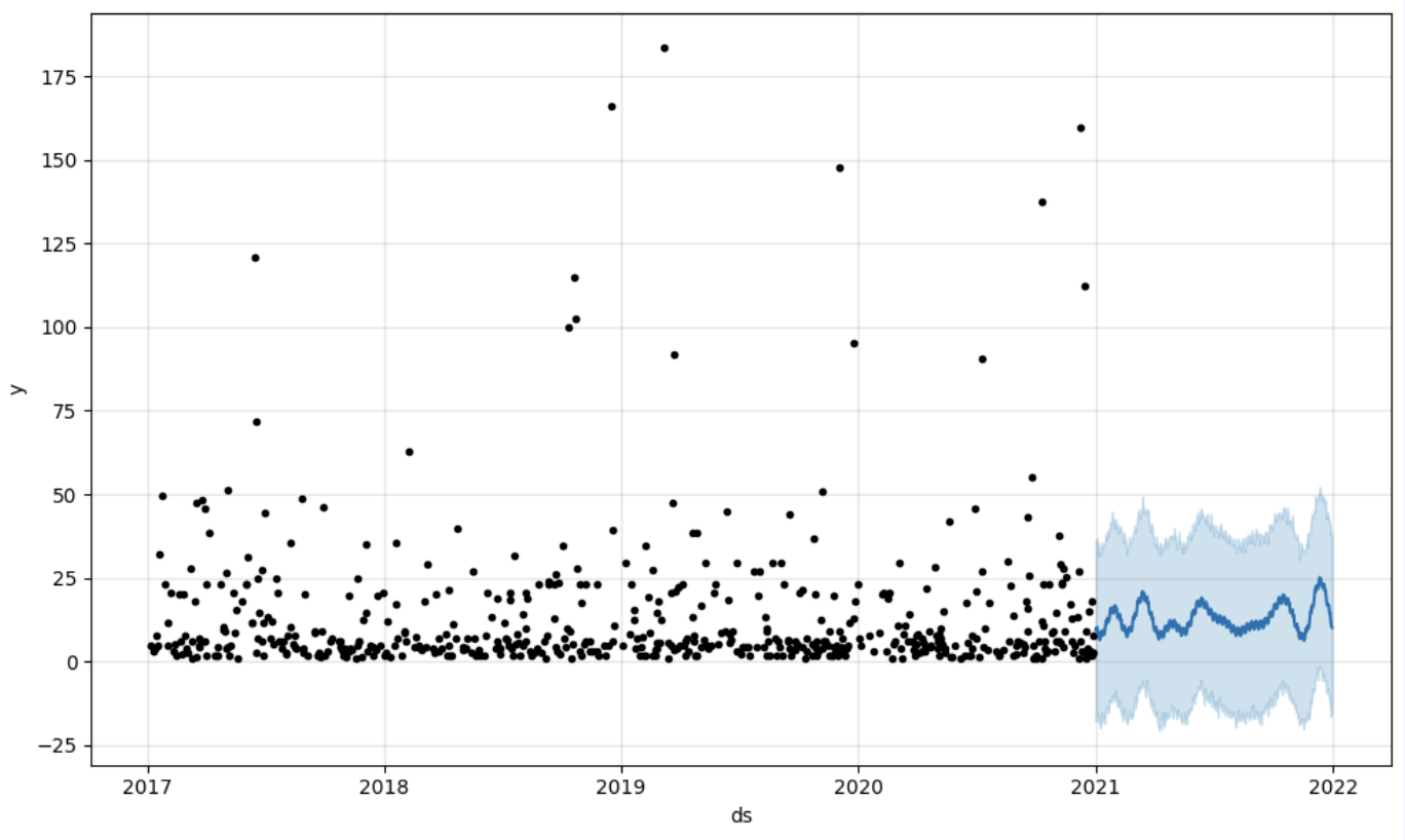
And then we create another dataframe to accomodate our prediction and display it on the graph

# Create a future dataframe for forecasting
future = pd.DataFrame()
future['ds'] = pd.date_range(start='2021-01-01', end='2021-12-31', freq='D')

# Make predictions
forecast = model.predict(future)
fig = model.plot(forecast)
fig.show()

Output:

Step 5: Writeback

Once we've got our prediction in place we can then put it back to the data warehouse and add an aggregate to our semantic model to reflect it for other consumers. The prediction would be available through any other BI tool for BI analysts and business users.
The prediction itself will be placed into our data warehouse and stored there.

from atscale.db.connections import Iris
db = Iris(
    username,
    host,
    namespace,
    driver,
    schema, 
    port=1972,
    password=None, 
    warehouse_id=None
    )

data_model.writeback(dbconn=db,
                    table_name= 'SalesPrediction',
                    DataFrame = forecast)

data_model.create_aggregate_feature(dataset_name='SalesPrediction',
                                    column_name='SalesForecasted',
                                    name='sum_sales_forecasted',
                                    aggregation_type='SUM')

Fin

That is it!
Good luck with your predictions!