Fast Automatic ML Hyperparameter tuning Using Optuna (w. MLflow model registry and IRIS DB)
This article presents a straightforward approach to automatically and efficiently tune hyperparameters for machine learning models using Optuna as the optimisation framework. We explore how to use both Optuna’s native storage options and InterSystems IRIS as a database backend to track the progress of hyperparameter searches. We also show how MLflow can be used to monitor experiments and manage models through its tracking and model registry UI.
This article is based on this Kaggle Notebook, which you can run and directly edit yourself.
When training ML models, the choice of hyperparameters can strongly influence performance. They are not the only factor, but they can significantly affect both convergence and generalisation.
Tuning hyperparameters manually takes a lot of effort. This is especially true because hyperparameters interact with each other, so tuning them independently is usually not enough. For example, higher regularisation may require a lower learning rate for more stable optimization. A more complex model may require stronger regularization to avoid overfitting, but at the same time, a very small learning rate on a complex model can make learning too slow.
Optuna is an MIT-licensed open source library, which allows commercial use, that automates hyperparameter search for ML models developed with the most popular frameworks such as scikit-learn, PyTorch, TensorFlow, and LightGBM. It works by defining a search space and an objective metric to either minimize or maximize. Optuna then explores the search space efficiently to find well-performing configurations.
Here we use Optuna to tune a LightGBM model on a dummy dataset and show how to scale the search using shared database storage. We will also use MLflow for experiment tracking and model registry, and IRIS DB as a possible Optuna storage backend for concurrent studies.
We will use the California Housing dataset, commonly used in ML examples, to populate IRIS tables and run the tuning workflow.
Note: For the last bit, you will need an existing IRIS instance that you can connect to. I am using the one created with Docker by running the docker-compose file from this repo. I am also using the environment variables and requirements.txt from that repository, together with Python 3.12.
import os
import dotenv
import sklearn
import pandas as pd
import sqlalchemy
from sqlalchemy import create_engine
import optuna
import lightgbm as lgb
from sklearn.model_selection import cross_val_score
from sklearn.model_selection import KFold
import seaborn as sns
import matplotlib.pyplot as plt
import datetime as dt
import seaborn as sns
import matplotlib.pyplot as plt


dotenv.load_dotenv()

# Connection String to Existing IRIS Database
server = os.getenv("IRIS_SERVER")
port = os.getenv("IRIS_PORT") # Standard InterSystems superserver port
namespace = os.getenv("IRIS_NAMESPACE")
username = os.getenv("IRIS_USERNAME")
password = os.getenv("IRIS_PASSWORD")

print(f"pandas version: {pd.__version__}")
print(f"sklearn version: {sklearn.__version__}")
print(f"sqlalchemy version: {sqlalchemy.__version__}")
print(f"optuna version: {optuna.__version__}")
print(f"lightgbm version: {lgb.__version__}")
print(f"seaborn version: {sns.__version__}")
print(f"matplotlib version: {plt.matplotlib.__version__}")
pandas version: 2.3.3
sklearn version: 1.8.0
sqlalchemy version: 2.0.46
optuna version: 4.8.0
lightgbm version: 4.6.0
seaborn version: 0.13.2
matplotlib version: 3.10.8
Quick Intro to Optuna
Optuna is a hyperparameter optimization framework that speeds up tuning by training multiple model configurations and learning from their results. It provides:
- Efficient sampling strategies, such as TPE, to focus on promising regions of the search space
- Pruning strategies to stop unpromising trials early
- Support for distributed optimization through shared storage
- Visualization tools to understand the search space and parameter importance
For a richer intro to Optuna, see this video
Optuna to Avoid Endless Hyperparameter Tuning:
A practical approach to efficiently find good hyperparameters is:
- Run an initial broad search to identify reasonable ranges and baseline parameters. In a CT pipeline, this would usually happen during the experimentation phase.
- Run a more focused Optuna search over the most promising ranges. In a CT pipeline, this can be repeated when there is data drift, model degradation, or a significant change in the dataset.
Important! Hyperparameter tuning must use an appropriate validation setup. Otherwise, we may only find the configuration that best overfits the validation split, rather than one that generalizes well to the dataset at hand.
Loading Dataset
The cell below loads scikit-learn's fetch_california_housing dataset, and changes the column names to snake case.
# Load California Housing Dataset
X,y = sklearn.datasets.fetch_california_housing(return_X_y=True,as_frame=True)
X.columns = [col.replace(" ", "_") for col in X.columns]
y.name = "median_house_value"
df = X.copy()
df[y.name] = y
Model Definition and Training
Choosing the right K-fold Split
It is essential to choose the right cross-validation strategy. This depends on the task, whether it is regression or classification, whether the target is imbalanced, whether the order of samples matters, and whether there are groups in the data. For example, if multiple rows belong to the same patient, we may want to avoid having samples from the same patient appear in both training and validation splits.
Refer to this summary of the options available in SKlearn for further guidance.
For simplicity, we can use the following decision rules:
if time_order_matters:
    use TimeSeriesSplit   # no shuffle equivalent
else:
    if groups_exist:
        if classification and classes_are_imbalanced:
            use StratifiedGroupKFold   # (no shuffle equivalent)
        else:
            use GroupKFold             # → or GroupShuffleSplit
    else:
        if classification and classes_are_imbalanced:
            use StratifiedKFold        # → or StratifiedShuffleSplit
        else:
            use KFold                  # → or ShuffleSplit
crossvalstrategy = KFold(n_splits=3, shuffle=True, random_state=42)
Hyperparemeter Search with Optuna
After choosing the model, in this case LightGBM, we define the hyperparameters that we want to tune and the metric that we want to optimize.
The cells in this section can be run multiple times until we reach a satisfactory performance level. The variables marked as tweakable are the ones we are likely to adjust between studies.
The general process is:
- Run an initial study with a broad search space.
- Inspect the best trials, parameter importance, and search-space plots.
- Use those results to define narrower and more promising ranges.
- Run a new study over the refined search space.
Since this is a regression task, we use mean squared error as the metric to minimize. The metric is evaluated using the cross-validation strategy defined above.
Note: When storage=storage_url points to a supported database, such as SQLite or InterSystems IRIS, Optuna automatically creates the tables needed to track studies, trials, parameters, and results. Each study is identified by its study_name. If the same study name and database are reused with load_if_exists=True, Optuna resumes from the existing study instead of starting from scratch.
This shared storage is also what enables concurrent optimization: multiple processes, or even multiple machines, can connect to the same database and contribute trials to the same study.
NUM_TRIALS = 20 # Tweak

os.environ["LOKY_MAX_CPU_COUNT"] = str(os.cpu_count())

def objective(trial):
    param = {
        "learning_rate": trial.suggest_float("learning_rate", 0.001, 0.2,log=True), # Tweak
        "max_depth": trial.suggest_int("max_depth", 3, 50), # Tweak
        "n_estimators": trial.suggest_int("n_estimators", 50, 1000), # Tweak
        "num_leaves": trial.suggest_categorical("num_leaves", [16, 31, 63, 127, 255]),
        "lambda_l2": trial.suggest_float("lambda_l2", 1e-8, 10.0, log=True), # Tweak
        "max_bin": trial.suggest_categorical("max_bin", [63, 127, 255])
    }

    model = lgb.LGBMRegressor(**param)

    scores = cross_val_score(model, X, y,
                            cv=crossvalstrategy,
                            scoring="neg_mean_squared_error",
                            n_jobs=-1)
    return -scores.mean()


study = optuna.create_study(study_name=f"lightgbm_hyperparam_tuning_{dt.datetime.now().strftime('%Y-%m-%d_%H-%M-%S')}",
                            direction="minimize",
                            # storage=storage_url,
                            load_if_exists=True,
                            sampler=optuna.samplers.TPESampler(seed=42),)
study.optimize(objective, n_trials=NUM_TRIALS, show_progress_bar=True, n_jobs=1)
best_params = study.best_params
print(f"\nBest parameters: {best_params}")
print(f"\nBest performance: {study.best_value}")
[32m[I 2026-05-13 15:58:38,618][0m A new study created in memory with name: lightgbm_hyperparam_tuning_2026-05-13_15-58-38[0m


  0%|          | 0/20 [00:00<?, ?it/s]


[32m[I 2026-05-13 15:59:02,770][0m Trial 0 finished with value: 0.22124664870518 and parameters: {'learning_rate': 0.00727491708802781, 'max_depth': 48, 'n_estimators': 746, 'num_leaves': 255, 'lambda_l2': 0.002570603566117598, 'max_bin': 255}. Best is trial 0 with value: 0.22124664870518.[0m
[32m[I 2026-05-13 15:59:06,986][0m Trial 1 finished with value: 0.2059125561807643 and parameters: {'learning_rate': 0.0823143373099555, 'max_depth': 13, 'n_estimators': 222, 'num_leaves': 63, 'lambda_l2': 0.0032112643094417484, 'max_bin': 255}. Best is trial 1 with value: 0.2059125561807643.[0m
[32m[I 2026-05-13 15:59:13,470][0m Trial 2 finished with value: 0.25714400572802726 and parameters: {'learning_rate': 0.01120548642504815, 'max_depth': 40, 'n_estimators': 239, 'num_leaves': 127, 'lambda_l2': 3.850031979199519e-08, 'max_bin': 127}. Best is trial 1 with value: 0.2059125561807643.[0m
[32m[I 2026-05-13 15:59:22,415][0m Trial 3 finished with value: 0.26413921215873515 and parameters: {'learning_rate': 0.0050225633119947675, 'max_depth': 7, 'n_estimators': 700, 'num_leaves': 255, 'lambda_l2': 2.133142332373004e-06, 'max_bin': 63}. Best is trial 1 with value: 0.2059125561807643.[0m
[32m[I 2026-05-13 15:59:28,245][0m Trial 4 finished with value: 0.20942294704047681 and parameters: {'learning_rate': 0.01811326544803337, 'max_depth': 11, 'n_estimators': 972, 'num_leaves': 31, 'lambda_l2': 6.257956190096665e-08, 'max_bin': 255}. Best is trial 1 with value: 0.2059125561807643.[0m
[32m[I 2026-05-13 15:59:54,053][0m Trial 5 finished with value: 0.22529793459324102 and parameters: {'learning_rate': 0.007840758945457348, 'max_depth': 16, 'n_estimators': 838, 'num_leaves': 255, 'lambda_l2': 4.6876566400928895e-08, 'max_bin': 63}. Best is trial 1 with value: 0.2059125561807643.[0m
[32m[I 2026-05-13 15:59:57,575][0m Trial 6 finished with value: 0.6243686001512612 and parameters: {'learning_rate': 0.0010296901472345186, 'max_depth': 42, 'n_estimators': 722, 'num_leaves': 31, 'lambda_l2': 0.5860448217200517, 'max_bin': 63}. Best is trial 1 with value: 0.2059125561807643.[0m
[32m[I 2026-05-13 16:00:01,328][0m Trial 7 finished with value: 0.25616396880444836 and parameters: {'learning_rate': 0.005194929407101736, 'max_depth': 18, 'n_estimators': 743, 'num_leaves': 31, 'lambda_l2': 0.0703178263660987, 'max_bin': 127}. Best is trial 1 with value: 0.2059125561807643.[0m
[32m[I 2026-05-13 16:00:02,230][0m Trial 8 finished with value: 0.4328137375744699 and parameters: {'learning_rate': 0.015952322469109693, 'max_depth': 23, 'n_estimators': 74, 'num_leaves': 63, 'lambda_l2': 1.4726456718740824, 'max_bin': 255}. Best is trial 1 with value: 0.2059125561807643.[0m
[32m[I 2026-05-13 16:00:03,606][0m Trial 9 finished with value: 0.5036899804922363 and parameters: {'learning_rate': 0.0033610226697378754, 'max_depth': 6, 'n_estimators': 325, 'num_leaves': 31, 'lambda_l2': 0.1710207048797339, 'max_bin': 127}. Best is trial 1 with value: 0.2059125561807643.[0m
[32m[I 2026-05-13 16:00:07,940][0m Trial 10 finished with value: 0.21142577467959092 and parameters: {'learning_rate': 0.14804113057514628, 'max_depth': 30, 'n_estimators': 458, 'num_leaves': 63, 'lambda_l2': 3.757350306893132e-05, 'max_bin': 255}. Best is trial 1 with value: 0.2059125561807643.[0m
[32m[I 2026-05-13 16:00:11,156][0m Trial 11 finished with value: 0.2017814916171883 and parameters: {'learning_rate': 0.08309297264998405, 'max_depth': 12, 'n_estimators': 950, 'num_leaves': 16, 'lambda_l2': 0.0008326596975497944, 'max_bin': 255}. Best is trial 11 with value: 0.2017814916171883.[0m
[32m[I 2026-05-13 16:00:12,488][0m Trial 12 finished with value: 0.20764432653610213 and parameters: {'learning_rate': 0.10507813096831281, 'max_depth': 28, 'n_estimators': 508, 'num_leaves': 16, 'lambda_l2': 0.0016316751769423123, 'max_bin': 255}. Best is trial 11 with value: 0.2017814916171883.[0m
[32m[I 2026-05-13 16:00:12,862][0m Trial 13 finished with value: 0.3044026543083153 and parameters: {'learning_rate': 0.054273532006916266, 'max_depth': 3, 'n_estimators': 131, 'num_leaves': 16, 'lambda_l2': 6.119264662645272e-05, 'max_bin': 255}. Best is trial 11 with value: 0.2017814916171883.[0m
[32m[I 2026-05-13 16:00:16,388][0m Trial 14 finished with value: 0.20646055020810183 and parameters: {'learning_rate': 0.041057846227823123, 'max_depth': 14, 'n_estimators': 366, 'num_leaves': 63, 'lambda_l2': 0.007230065446525416, 'max_bin': 255}. Best is trial 11 with value: 0.2017814916171883.[0m
[32m[I 2026-05-13 16:00:18,008][0m Trial 15 finished with value: 0.21268042685192567 and parameters: {'learning_rate': 0.04807456550053136, 'max_depth': 21, 'n_estimators': 604, 'num_leaves': 16, 'lambda_l2': 6.458243615671745e-06, 'max_bin': 255}. Best is trial 11 with value: 0.2017814916171883.[0m
[32m[I 2026-05-13 16:00:28,022][0m Trial 16 finished with value: 0.21844697644015332 and parameters: {'learning_rate': 0.18423283160212306, 'max_depth': 10, 'n_estimators': 992, 'num_leaves': 127, 'lambda_l2': 9.015211997542714, 'max_bin': 255}. Best is trial 11 with value: 0.2017814916171883.[0m
[32m[I 2026-05-13 16:00:29,373][0m Trial 17 finished with value: 0.20797590828555537 and parameters: {'learning_rate': 0.08294987485804219, 'max_depth': 33, 'n_estimators': 188, 'num_leaves': 63, 'lambda_l2': 0.018231434623139052, 'max_bin': 255}. Best is trial 11 with value: 0.2017814916171883.[0m
[32m[I 2026-05-13 16:00:30,247][0m Trial 18 finished with value: 0.23633039578627624 and parameters: {'learning_rate': 0.02831149820738454, 'max_depth': 24, 'n_estimators': 355, 'num_leaves': 16, 'lambda_l2': 0.00012197971292668617, 'max_bin': 127}. Best is trial 11 with value: 0.2017814916171883.[0m
[32m[I 2026-05-13 16:00:35,660][0m Trial 19 finished with value: 0.21720640666066582 and parameters: {'learning_rate': 0.07858633974467637, 'max_depth': 13, 'n_estimators': 879, 'num_leaves': 63, 'lambda_l2': 0.0007188574432995588, 'max_bin': 63}. Best is trial 11 with value: 0.2017814916171883.[0m

Best parameters: {'learning_rate': 0.08309297264998405, 'max_depth': 12, 'n_estimators': 950, 'num_leaves': 16, 'lambda_l2': 0.0008326596975497944, 'max_bin': 255}

Best performance: 0.2017814916171883
Below we inspect the best-performing trials from the study. This gives us a quick view of which hyperparameter combinations performed best and helps guide future searches:
trials_df = study.trials_dataframe()
trials_df = trials_df.sort_values("value")
trials_df = trials_df.loc[:, trials_df.columns.str.contains("params|value")]
top_trials_df = trials_df.head(10)

display(top_trials_df)
display(top_trials_df.describe())
| value | params_lambda_l2 | params_learning_rate | params_max_bin | params_max_depth | params_n_estimators | params_num_leaves | |
|---|---|---|---|---|---|---|---|
| 11 | 0.201781 | 8.326597e-04 | 0.083093 | 255 | 12 | 950 | 16 |
| 1 | 0.205913 | 3.211264e-03 | 0.082314 | 255 | 13 | 222 | 63 |
| 14 | 0.206461 | 7.230065e-03 | 0.041058 | 255 | 14 | 366 | 63 |
| 12 | 0.207644 | 1.631675e-03 | 0.105078 | 255 | 28 | 508 | 16 |
| 17 | 0.207976 | 1.823143e-02 | 0.082950 | 255 | 33 | 188 | 63 |
| 4 | 0.209423 | 6.257956e-08 | 0.018113 | 255 | 11 | 972 | 31 |
| 10 | 0.211426 | 3.757350e-05 | 0.148041 | 255 | 30 | 458 | 63 |
| 15 | 0.212680 | 6.458244e-06 | 0.048075 | 255 | 21 | 604 | 16 |
| 19 | 0.217206 | 7.188574e-04 | 0.078586 | 63 | 13 | 879 | 63 |
| 16 | 0.218447 | 9.015212e+00 | 0.184233 | 255 | 10 | 992 | 127 |
| value | params_lambda_l2 | params_learning_rate | params_max_bin | params_max_depth | params_n_estimators | params_num_leaves | |
|---|---|---|---|---|---|---|---|
| count | 10.000000 | 1.000000e+01 | 10.000000 | 10.000000 | 10.000000 | 10.000000 | 10.000000 |
| mean | 0.209896 | 9.047112e-01 | 0.087154 | 235.800000 | 18.500000 | 613.900000 | 52.100000 |
| std | 0.005155 | 2.849745e+00 | 0.049444 | 60.715731 | 8.759122 | 313.844424 | 34.252169 |
| min | 0.201781 | 6.257956e-08 | 0.018113 | 63.000000 | 10.000000 | 188.000000 | 16.000000 |
| 25% | 0.206756 | 2.078945e-04 | 0.055703 | 255.000000 | 12.250000 | 389.000000 | 19.750000 |
| 50% | 0.208699 | 1.232167e-03 | 0.082632 | 255.000000 | 13.500000 | 556.000000 | 63.000000 |
| 75% | 0.212367 | 6.225365e-03 | 0.099582 | 255.000000 | 26.250000 | 932.250000 | 63.000000 |
| max | 0.218447 | 9.015212e+00 | 0.184233 | 255.000000 | 33.000000 | 992.000000 | 127.000000 |
After the first broad search, we can estimate which hyperparameters had the strongest impact on performance. This helps us decide which parameters deserve a more focused search in the next study.
The cell below calculates the importance score for each hyperparameter on a scale from 0 to 1. Higher values indicate parameters that had more influence on the objective metric in this study.
param_importance_dict = optuna.importance.get_param_importances(study)

plt.figure(figsize=(10, 6))
sns.barplot(x=list(param_importance_dict.values()), y=list(param_importance_dict.keys()))
plt.xlabel('Importance Score')
plt.ylabel('Hyperparameter')
plt.title('Hyperparameter Importance')
plt.tight_layout()
plt.grid()
plt.show()
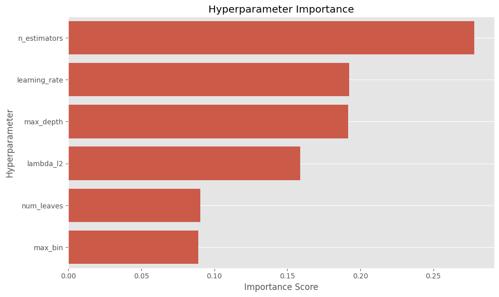
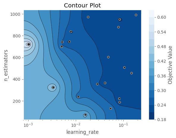
From the plot above, we can identify the most relevant hyperparameters. Next, we choose how many of the top parameters we want to compare. In this example, we select the two most important ones.
The contour plot below helps us visualize how these two parameters interact and which regions of the search space produced better results. We can use this to define narrower ranges for future studies.
numparamstocompare = 2
best2params = [k for k, v in sorted(param_importance_dict.items(), key=lambda x: x[1])[-numparamstocompare:]]
optuna.visualization.matplotlib.plot_contour(study, params=best2params)
Concurrent studies to speed up Hyperparameter exploration
Every time we test a set of hyperparameters, we should evaluate it properly using cross-validation to avoid selecting a model that just overfits to a particular train/validation split. This means training as many models as the number of folds we choose.
For example, using 5-fold or 10-fold cross-validation implies training 5–10 models per hyperparameter configuration. There is no strict rule for the number of folds, but 5 or 10 are commonly used depending on how expensive each model is to train. As a result, evaluating each set of hyperparameters becomes 5–10 times more time-consuming, and this cost increases further as the dataset grows.
For this reason, we want to accelerate the hyperparameter search. One way to do this is by running multiple processes, each working on the same Optuna study and exploring the same search space in parallel. If a machine has 16 cores, we can run up to 16 workers concurrently, which can significantly reduce the total optimization time (although not always perfectly linearly due to overhead and coordination between workers).
An important advantage of Optuna is that if all workers point to a common storage database, the study is shared across processes. Optuna will create and manage the required tables in the database, and all workers will contribute trials to the same study. This means that:
- Workers generally avoid evaluating identical hyperparameter configurations
- Completed trials from all workers are used to guide future sampling
- The search becomes more efficient over time as more results are collected
By default, you can specify "sqlite:///optuna_lgbm.db" as the storage parameter, and Optuna will create a local database for the study. The same approach can also be extended to a centralized database such as InterSystems IRIS, enabling distributed hyperparameter tuning across multiple machines.
Optuna's native Concurrency + MLflow model registry
We can combine Optuna for hyperparameter tuning and MLflow for experiment tracking and model registry. This way, we can leverage the same MLflow model registry capabilities shown in this repo.
One of the main advantages of Optuna is how easy it is to scale hyperparameter tuning across processes or even across machines. We can run the same optimization study from different machines, and as long as all of them point to the same storage database, all workers will contribute trials to the same study. As trials finish, Optuna can use the accumulated results to guide future samples.
In the example below, we run multiple workers against the same Optuna study. Running this as a separate Python script, not in a standard Jupyter notebook, allows parallel hyperparameter tuning with MLflow tracking. MLflow keeps track of the parent run, each child trial run, the final best parameters, the best cross-validation score, and the final trained model.
The cell below ran 3200 trials in 25 minutes on a Windows laptop with 16 cores, using 16 workers with 200 trials each. Each trial used 3 cross-validation splits.
import os
import dotenv
import optuna
import lightgbm as lgb
import multiprocessing as mp
import mlflow
import mlflow.lightgbm
from mlflow.models import infer_signature
import numpy as np
from sklearn.model_selection import cross_val_score, KFold
from sklearn.datasets import fetch_california_housing
import datetime as dt

dotenv.load_dotenv()

STORAGE_URL = "sqlite:///optuna_lgbm.db"  # for local testing


# Hyperparameter tuning configuration
NUM_WORKERS = min(16, mp.cpu_count())
NUM_TRIALS_PER_WORKER = 200
BASE_SEED = 42
NUM_CV_SPLITS = 3 # 5 or 10 would be better
EXPERIMENT_NAME = "LightGBM Hyperparameter Tuning with Optuna and MLflow"
crossvalstrategy = KFold(n_splits=NUM_CV_SPLITS, shuffle=True, random_state=BASE_SEED)

# Load dataset
X, y = fetch_california_housing(return_X_y=True, as_frame=True)
X.columns = [col.replace(" ", "_") for col in X.columns]
y.name = "median_house_value"

def objective(trial):
    params = {
        "learning_rate": trial.suggest_float("learning_rate", 0.001, 0.2, log=True),  # CHANGEABLE
        "max_depth": trial.suggest_int("max_depth", 3, 50),  # CHANGEABLE
        "n_estimators": trial.suggest_int("n_estimators", 50, 1000),  # CHANGEABLE
        "num_leaves": trial.suggest_categorical("num_leaves", [16, 31, 63, 127, 255]),
        "lambda_l2": trial.suggest_float("lambda_l2", 1e-8, 10.0, log=True),  # CHANGEABLE
        "max_bin": trial.suggest_categorical("max_bin", [63, 127, 255]),
        "random_state": BASE_SEED,
        "verbosity": -1,
        "n_jobs": 1,
    }

    parent_run_id = os.getenv("MLFLOW_PARENT_RUN_ID")

    with mlflow.start_run(
        run_name=f"trial_{trial.number}",
        nested=True,
        parent_run_id=parent_run_id,
        # tags={"mlflow.parentRunId": parent_run_id} if parent_run_id else None,
    ) as child_run:

        mlflow.log_params(params)

        model = lgb.LGBMRegressor(**params)

        scores = cross_val_score(
            model,
            X,
            y,
            cv=crossvalstrategy,
            scoring="neg_mean_squared_error",
            n_jobs=1,
        )

        crossval_score = -scores.mean()

        # Log current trial's error metric
        mlflow.log_metrics({"cv_mse_mean": crossval_score})
        for fold_idx, score in enumerate(scores):
            mlflow.log_metric(f"fold_{fold_idx}_mse", -score)

        # Make it easy to retrieve the best-performing child run later
        trial.set_user_attr("run_id", child_run.info.run_id)

        return crossval_score


def run_worker(args):
    worker_id, study_name, parent_run_id = args
    mlflow.set_tracking_uri(os.getenv("MLFLOW_TRACKING_URI"))
    mlflow.set_experiment(EXPERIMENT_NAME)
    os.environ["MLFLOW_PARENT_RUN_ID"] = parent_run_id

    study = optuna.load_study(
        study_name=study_name,
        storage=STORAGE_URL,
        sampler=optuna.samplers.TPESampler(seed=BASE_SEED+worker_id),
        )
    study.optimize(
        objective,
        n_trials=NUM_TRIALS_PER_WORKER,
        show_progress_bar=False,
        n_jobs=1,
    )
    return worker_id


if __name__ == "__main__":

    # MLflow setup
    datetime_str = dt.datetime.now().strftime("%Y-%m-%d %H:%M")
    RUN_NAME = f"parent_{datetime_str}"
    STUDY_NAME = f"optuna_{datetime_str}"
    tracking_uri = os.getenv("MLFLOW_TRACKING_URI")
    mlflow.set_tracking_uri(tracking_uri)
    mlflow.set_experiment(EXPERIMENT_NAME)
    experiment = mlflow.get_experiment_by_name(EXPERIMENT_NAME)
    experiment_id = experiment.experiment_id


    with mlflow.start_run(run_name=RUN_NAME, log_system_metrics=True) as parent_run:
        parent_run_id = parent_run.info.run_id
        os.environ["MLFLOW_PARENT_RUN_ID"] = parent_run_id

        optuna.create_study(
            direction="minimize",
            study_name=STUDY_NAME,
            storage=STORAGE_URL,
            load_if_exists=False,
        )

        mlflow.log_params({
            "n_trials": NUM_TRIALS_PER_WORKER * NUM_WORKERS,
            "num_workers": NUM_WORKERS,
            "cv_n_splits": crossvalstrategy.n_splits,
            "seed": BASE_SEED,
            "study_name": STUDY_NAME,
        })

        worker_args = [
            (worker_id, STUDY_NAME, parent_run_id)
            for worker_id in range(NUM_WORKERS)
        ]
        with mp.Pool(processes=NUM_WORKERS) as pool:
            pool.map(run_worker, worker_args)

        study = optuna.load_study(
            study_name=STUDY_NAME,
            storage=STORAGE_URL,
        )

        best_params = study.best_trial.params
        best_value = study.best_value
        best_child_run_id = study.best_trial.user_attrs.get("run_id")

        mlflow.log_params({f"best_{k}": v for k, v in best_params.items()})
        mlflow.log_metric("best_cv_mse", float(best_value))

        if best_child_run_id:
            mlflow.log_param("best_child_run_id", best_child_run_id)

        # Train final model on full dataset with best hyperparameters. Important: keep same seed
        final_model = lgb.LGBMRegressor(
            **best_params,
            random_state=BASE_SEED,
            verbosity=-1,
            n_jobs=1,
        )
        final_model.fit(X, y)
        input_sample = X.sample(100, random_state=BASE_SEED)
        signature = infer_signature(input_sample, final_model.predict(input_sample))
        mlflow.lightgbm.log_model(
            lgb_model=final_model,
            name="best_model",
            signature=signature,
            input_example=X.head(5),
        )
The code above works as a proof of concept when working across different machines. Each machine or process can point to the same shared Optuna storage database and contribute trials to the same study.
However, if we are using a single PC, the simpler version below is usually preferable. It runs the same study with parallel jobs controlled by Optuna's n_jobs parameter. This approach is simpler and can achieve similar performance, although the exact trials and final best model are not guaranteed to be identical to the multiprocessing version.
The code below also ran 3200 trials, in this case in 27 minutes.
import os
import dotenv
import optuna
import lightgbm as lgb
import multiprocessing as mp
import mlflow
import mlflow.lightgbm
from mlflow.models import infer_signature
import numpy as np
from sklearn.model_selection import cross_val_score, KFold
from sklearn.datasets import fetch_california_housing
import datetime as dt

dotenv.load_dotenv()

STORAGE_URL = "sqlite:///optuna_lgbm.db"  # for local testing


# Hyperparameter tuning configuration
NUM_WORKERS = min(16, mp.cpu_count())
NUM_TRIALS_PER_WORKER = 200
BASE_SEED = 42
NUM_CV_SPLITS = 3 # 5 or 10 would be better
EXPERIMENT_NAME = "LightGBM Hyperparameter Tuning with Optuna and MLflow 2"
crossvalstrategy = KFold(n_splits=NUM_CV_SPLITS, shuffle=True, random_state=BASE_SEED)

# Load dataset
X, y = fetch_california_housing(return_X_y=True, as_frame=True)
X.columns = [col.replace(" ", "_") for col in X.columns]
y.name = "median_house_value"

def objective(trial):
    params = {
        "learning_rate": trial.suggest_float("learning_rate", 0.001, 0.2, log=True),  # CHANGEABLE
        "max_depth": trial.suggest_int("max_depth", 3, 50),  # CHANGEABLE
        "n_estimators": trial.suggest_int("n_estimators", 50, 1000),  # CHANGEABLE
        "num_leaves": trial.suggest_categorical("num_leaves", [16, 31, 63, 127, 255]),
        "lambda_l2": trial.suggest_float("lambda_l2", 1e-8, 10.0, log=True),  # CHANGEABLE
        "max_bin": trial.suggest_categorical("max_bin", [63, 127, 255]),
        "random_state": BASE_SEED,
        "verbosity": -1,
        "n_jobs": 1,
    }

    parent_run_id = os.getenv("MLFLOW_PARENT_RUN_ID")

    with mlflow.start_run(
        run_name=f"trial_{trial.number}",
        nested=True,
        parent_run_id=parent_run_id,
        # tags={"mlflow.parentRunId": parent_run_id} if parent_run_id else None,
    ) as child_run:

        mlflow.log_params(params)

        model = lgb.LGBMRegressor(**params)

        scores = cross_val_score(
            model,
            X,
            y,
            cv=crossvalstrategy,
            scoring="neg_mean_squared_error",
            n_jobs=1,
        )

        crossval_score = -scores.mean()

        # Log current trial's error metric
        mlflow.log_metrics({"cv_mse_mean": crossval_score})
        for fold_idx, score in enumerate(scores):
            mlflow.log_metric(f"fold_{fold_idx}_mse", -score)

        # Make it easy to retrieve the best-performing child run later
        trial.set_user_attr("run_id", child_run.info.run_id)

        return crossval_score


if __name__ == "__main__":

    # MLflow setup
    datetime_str = dt.datetime.now().strftime("%Y-%m-%d %H:%M")
    RUN_NAME = f"parent_{datetime_str}"
    STUDY_NAME = f"optuna_{datetime_str}"
    tracking_uri = os.getenv("MLFLOW_TRACKING_URI")
    mlflow.set_tracking_uri(tracking_uri)
    mlflow.set_experiment(EXPERIMENT_NAME)
    experiment = mlflow.get_experiment_by_name(EXPERIMENT_NAME)
    experiment_id = experiment.experiment_id


    with mlflow.start_run(run_name=RUN_NAME, log_system_metrics=True) as parent_run:
        parent_run_id = parent_run.info.run_id
        os.environ["MLFLOW_PARENT_RUN_ID"] = parent_run_id

        optuna.create_study(
            direction="minimize",
            study_name=STUDY_NAME,
            storage=STORAGE_URL,
            load_if_exists=False,
        )

        mlflow.log_params({
            "n_trials": NUM_TRIALS_PER_WORKER * NUM_WORKERS,
            "num_workers": NUM_WORKERS,
            "cv_n_splits": crossvalstrategy.n_splits,
            "seed": BASE_SEED,
            "study_name": STUDY_NAME,
        })

        study = optuna.load_study(
            study_name=STUDY_NAME,
            storage=STORAGE_URL,
        )
        study.optimize(
            objective,
            n_trials=NUM_TRIALS_PER_WORKER * NUM_WORKERS,
            show_progress_bar=False,
            n_jobs=NUM_WORKERS,
        )
        best_params = study.best_trial.params
        best_value = study.best_value
        best_child_run_id = study.best_trial.user_attrs.get("run_id")

        mlflow.log_params({f"best_{k}": v for k, v in best_params.items()})
        mlflow.log_metric("best_cv_mse", float(best_value))

        if best_child_run_id:
            mlflow.log_param("best_child_run_id", best_child_run_id)

        # Train final model on full dataset with best hyperparameters. Important: keep same seed
        final_model = lgb.LGBMRegressor(
            **best_params,
            random_state=BASE_SEED,
            verbosity=-1,
            n_jobs=NUM_WORKERS,
        )
        final_model.fit(X, y)
        input_sample = X.sample(100, random_state=BASE_SEED)
        signature = infer_signature(input_sample, final_model.predict(input_sample))
        mlflow.lightgbm.log_model(
            lgb_model=final_model,
            name="best_model",
            signature=signature,
            input_example=X.head(5),
        )
As a result of running either script, we get a parent run in MLflow with the final best model trained using the best hyperparameters found across the 3200 trials. The parent run also stores the best hyperparameters, the best cross-validation score, and the ID of the best child run. Each child run contains the parameters and metrics for one Optuna trial.
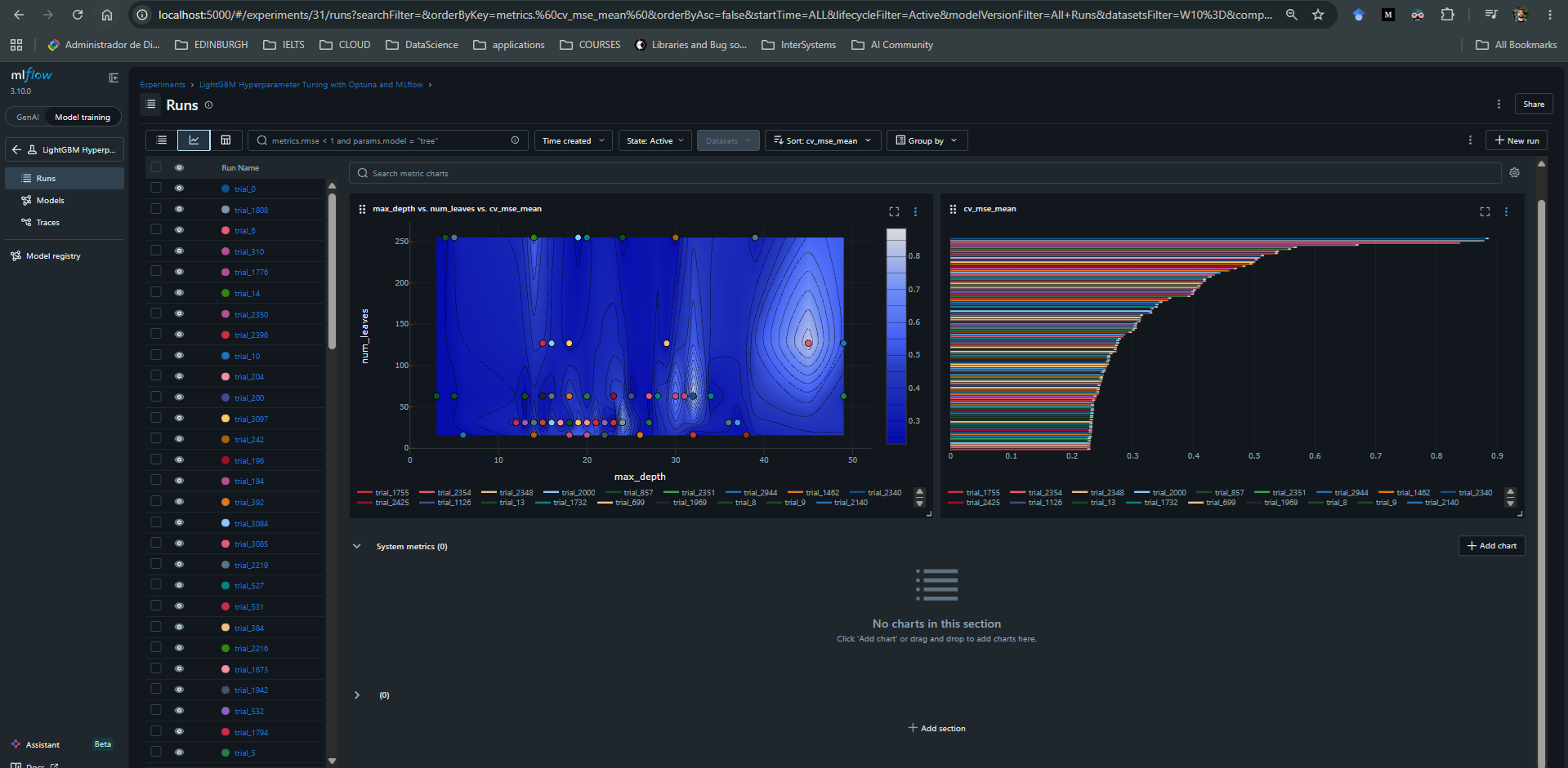
All of this can be explored in the MLflow UI, for example at http://localhost:5000/#/experiments, where we can inspect the parent run, compare child runs, and download or register the final model.
In the image below, we see two plots from MLflow's UI. On the left, we get a sense of the search space by comparing the mean cross-validation MSE across trials with different values of max_depth and num_leaves. On the right, we see the 100 worst models, meaning the trials with the highest mean squared error across cross-validation. The best found model achieved a score of approximately 0.199580.
Optuna Concurrency + IRIS DB
When trying to replicate the same process with IRIS DB as the Optuna storage backend, multiple issues arose when running more than 4 workers in parallel. This is likely related to how each worker process creates its own connection to IRIS and writes trial metadata concurrently to the same Optuna study.
The code below worked fine with up to 3 workers running at the same time. Another option is to keep a single Python process pointing to IRIS and set Optuna's n_jobs parameter to the number of concurrent jobs we want (just as we did above). This approach uses threads inside one process, which can be simpler from a database-connection perspective because it avoids multiple independent Python processes creating separate connections to IRIS.
However, this approach is not always equivalent to multiprocessing. Since Optuna's n_jobs uses threads, CPU-bound Python code can be limited by Python's GIL. In this specific example, most of the expensive work is done by LightGBM and scikit-learn routines, so threading may still provide useful speedup, but it may not scale the same way as true multiprocessing.
import os
import dotenv
import optuna
import lightgbm as lgb
import multiprocessing as mp
from sqlalchemy.pool import NullPool
from sklearn.model_selection import cross_val_score, KFold
from sklearn.datasets import fetch_california_housing
import datetime as dt

dotenv.load_dotenv()

NUM_WORKERS = min(8, mp.cpu_count())  # CHANGEABLE
NUM_TRIALS_PER_WORKER = 20  # CHANGEABLE
STUDY_NAME = f"IRIS_lightgbm_study_{dt.datetime.now().strftime('%Y-%m-%d_%H-%M-%S')}"  # CHANGEABLE
BASE_SEED = 42  # CHANGEABLE

server = os.getenv("IRIS_SERVER")
port = os.getenv("IRIS_PORT")
namespace = os.getenv("IRIS_NAMESPACE")
username = os.getenv("IRIS_USERNAME")
password = os.getenv("IRIS_PASSWORD")
STORAGE_URL = f"iris://{username}:{password}@{server}:{port}/{namespace}"
crossvalstrategy = KFold(n_splits=3, shuffle=True, random_state=BASE_SEED)

# Load Dataset
X, y = fetch_california_housing(return_X_y=True, as_frame=True)
X.columns = [col.replace(" ", "_") for col in X.columns]
y.name = "median_house_value"


def objective(trial):
    param = {
        "learning_rate": trial.suggest_float(
            "learning_rate", 0.001, 0.2, log=True
        ),  # CHANGEABLE
        "max_depth": trial.suggest_int("max_depth", 3, 50),  # CHANGEABLE
        "n_estimators": trial.suggest_int("n_estimators", 50, 1000),  # CHANGEABLE
        "num_leaves": trial.suggest_categorical("num_leaves", [16, 31, 63, 127, 255]),
        "lambda_l2": trial.suggest_float(
            "lambda_l2", 1e-8, 10.0, log=True
        ),  # CHANGEABLE
        "max_bin": trial.suggest_categorical("max_bin", [63, 127, 255]),
        "random_state": BASE_SEED,
        "verbosity": -1,
        "n_jobs": 1,
    }

    model = lgb.LGBMRegressor(**param)

    scores = cross_val_score(
        model,
        X,
        y,
        cv=crossvalstrategy,
        scoring="neg_mean_squared_error",
        n_jobs=1,
    )
    return -scores.mean()


def run_worker(args):

    worker_id, study_name, _ = args
    worker_storage = make_storage()
    study = optuna.load_study(
        study_name=study_name,
        storage=worker_storage,
        sampler=optuna.samplers.TPESampler(seed=BASE_SEED + worker_id),
    )
    study.optimize(
        objective, n_trials=NUM_TRIALS_PER_WORKER, show_progress_bar=False, n_jobs=1
    )
    return worker_id

def make_storage():
    return optuna.storages.RDBStorage(
        url=STORAGE_URL,
        engine_kwargs={
            "poolclass": NullPool,
            "connect_args": {
                "timeout": 30
            },  # Helps with heavy concurrent writes
        },
    )

if __name__ == "__main__":

    main_storage = make_storage()
    optuna.create_study(
        direction="minimize",
        study_name=STUDY_NAME,
        storage=main_storage,
        load_if_exists=False,
    )
    if hasattr(main_storage, "get_engine"):
        main_storage.get_engine().dispose()

    worker_args = [(worker_id,STUDY_NAME,None) for worker_id in range(NUM_WORKERS)]
    with mp.Pool(processes=NUM_WORKERS) as pool:
        results = pool.map(run_worker, worker_args)

    final_storage = make_storage()
    final_study = optuna.load_study(study_name=STUDY_NAME, storage=final_storage)
    print(
        f"\nOverall Best Value: {final_study.best_value}, Overall Best Params: {final_study.best_params}"
    )
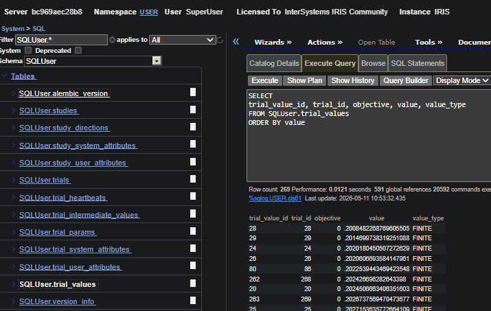
Optuna saves the study metadata in IRIS for future reference. This includes studies, trials, trial parameters, trial values, intermediate values, and related metadata in the Optuna storage tables created in IRIS.
For further performance analysis, we can query these tables directly or, preferably, load the study back through Optuna and use Optuna's built-in visualization and analysis tools to inspect the optimization history, parameter importance, and trial performance.
The image below shows the Optuna storage tables created in IRIS DB.