How to develop an InterSystems Adaptive Analytics (AtScale) cube

 

Today we will talk about Adaptive Analytics. This is a system that allows you to receive data from various sources with a relativistic data structure and create OLAP cubes based on this data. This system also provides the ability to filter and aggregate data and has mechanisms to speed up the work of analytical queries.

Let's take a look at the path that data takes from input to output in Adaptive Analytics. We will start by connecting to a data source -  our instance of IRIS. 

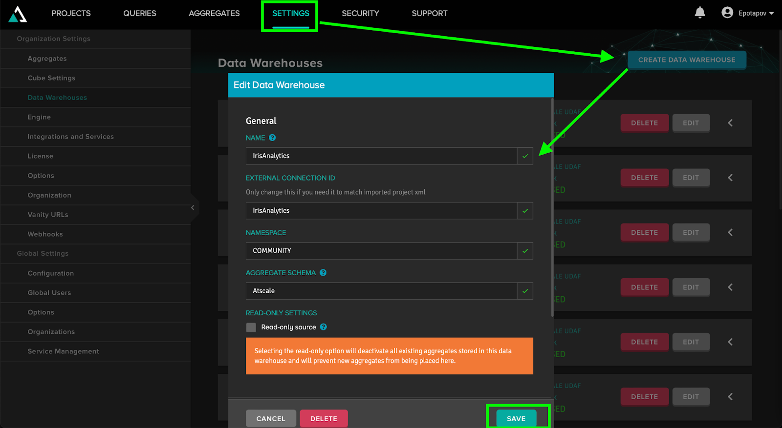
In order to create a connection to the source, you need to go to the Settings tab of the top menu and select the Data Warehouses section. Here we click the “Create Data Warehouse” button and pick “InterSystems IRIS” as the source. Next, we will need to fill in the Name and External Connection ID fields (use the name of our connection to do that), and the Namespace (corresponds to the desired Namespace in IRIS). Since we will talk about the Aggregate Schema and Custom Function Installation Mode fields later, we will leave them by default for now. 

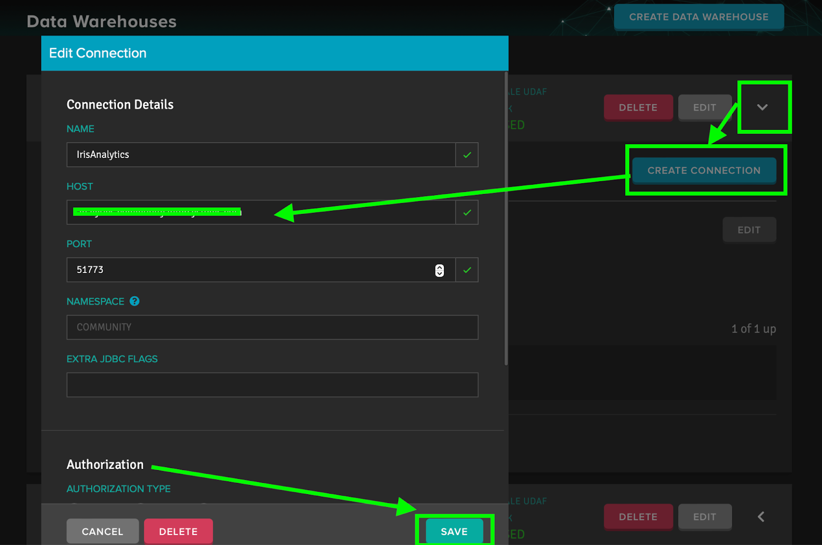
When Adaptive Analytics creates our Data Warehouse, we need to establish a connection with IRIS for it. To do this, open the Data Warehouse with a white arrow and click the “Create Connection” button. Here we should fill in the data of our IRIS server (host, port, username, and password) as well as the name of the connection. Please note that the Namespace is filled in automatically from the Data Warehouse and cannot be changed in the connection settings.

After the data has entered our system, it must be processed somewhere. To make it happen, we will create a project. The project processes data from only one connection. However, one connection can be involved in several projects. If you have multiple data sources for a report, you will need to create a project for each of them. 

All entity names in a project must be unique. The cubes in the project (more on them later) are interconnected not only by links explicitly configured by the user, but also if they use the same table from the data source.

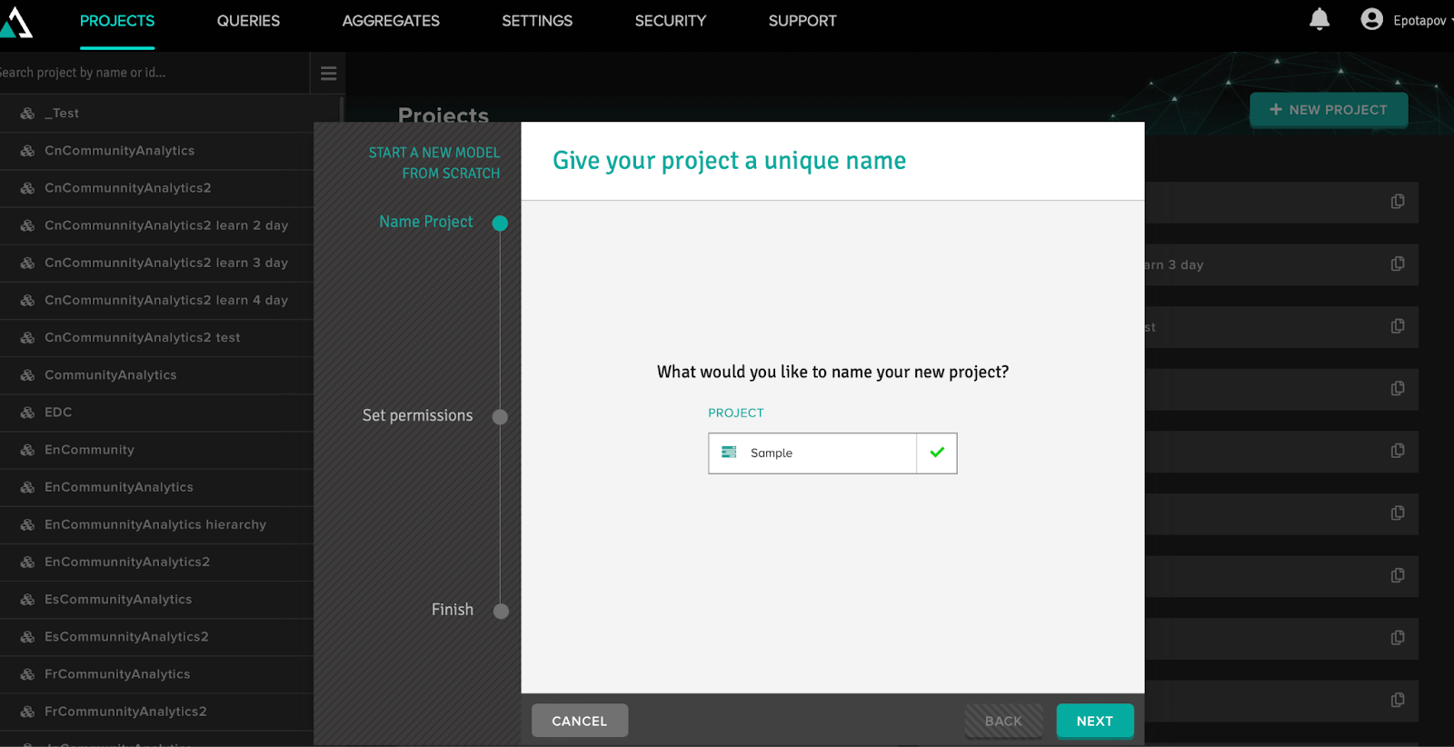
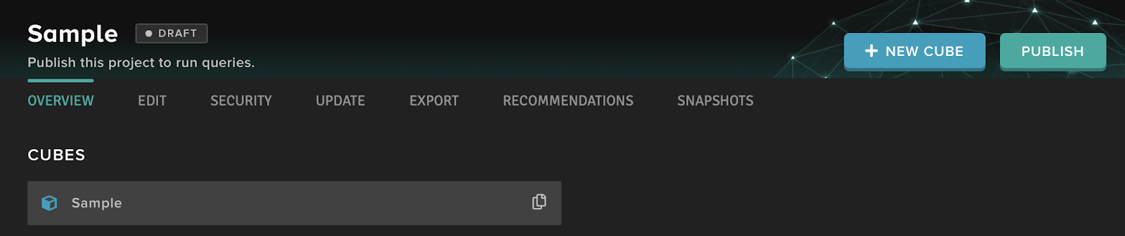
 To create a project, go to the Projects tab and click the “New Project” button. Now you can create OLAP cubes in the project. To do that, we will need to use the “New Cube” button, fill in the name of the cube and proceed to its development.

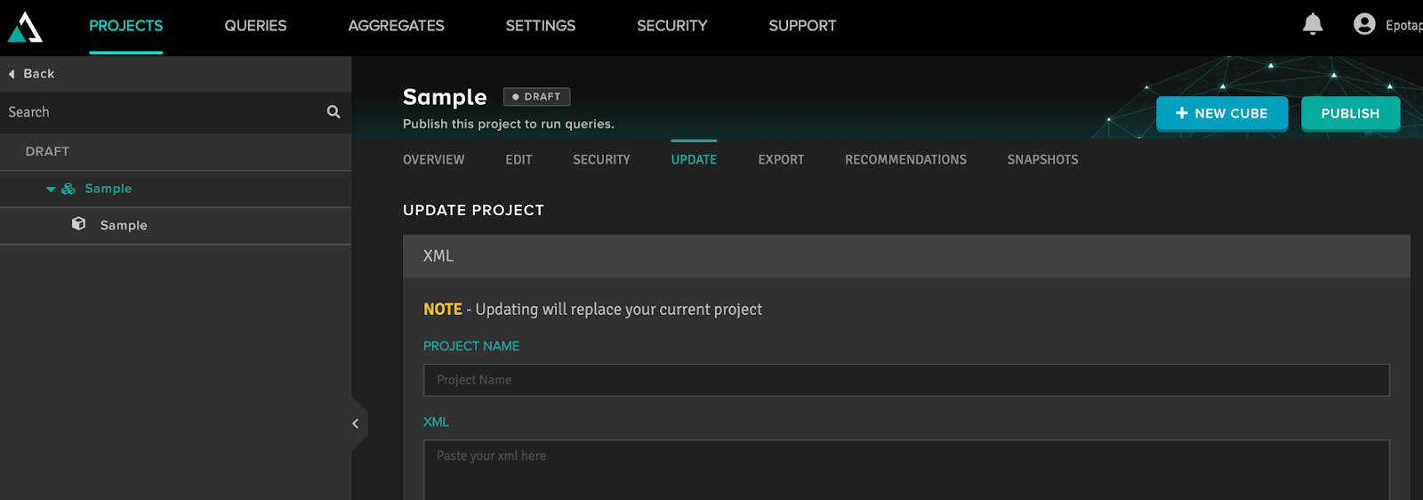
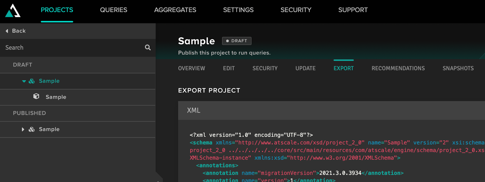
Let's dwell on the rest of the project's functionality. Under the name of the project, we can see a menu of tabs, out of which it is worth elaborating on the Update, Export, and Snapshots tabs. On the Export tab, we can save the project structure as an XML file. In this way, you can migrate projects from one Adaptive Analytics server to another or clone projects to connect to multiple data sources with the same structure. On the Update tab, we can insert text from the XML document and bring the cube to the structure that is described in this document. On the Snapshots tab, we can do version control of the project, switching between different versions if desired.

Now let's talk about what the Adaptive Analytics cube contains. Upon entering the cube, we are greeted by a description of its contents which shows us the type and number of entities that are present in it. To view its structure, press the “Enter model” button. It will bring you to the Cube Canvas tab, which contains all the data tables added to the cube, dimensions, and relationships between them. 

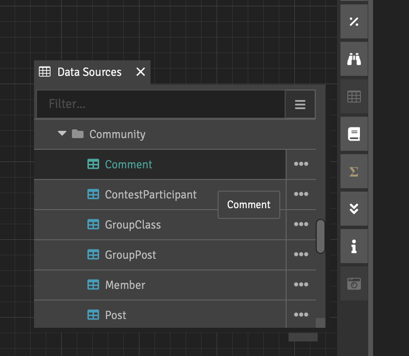
In order to get data into the cube, we need to go to the Data Sources tab on the right control panel. The icon of this tab looks like a tablet. Here we should click on the “hamburger” icon and select Remap Data Source. We select the data source we need by name. Congratulations, the data has arrived in the project and is now available in all its cubes. You can see the namespace of the IRIS structure on this tab and what the data looks like in the tables.

Now it’s time to  talk about each entity that makes up the structure of the cube.

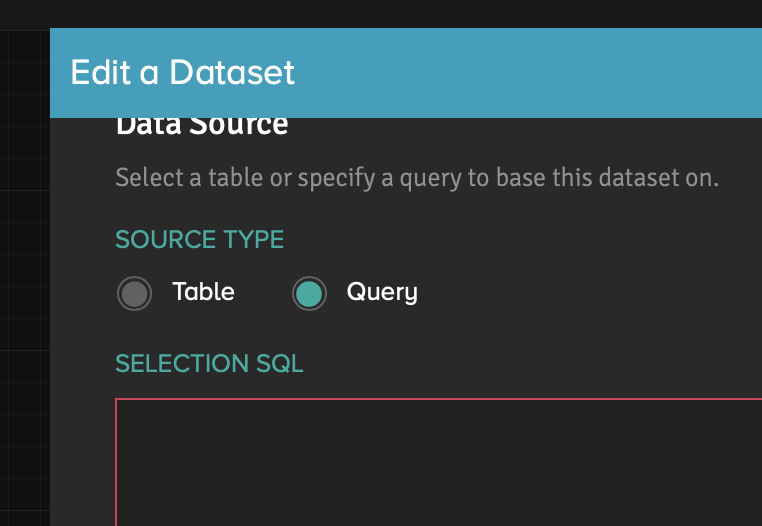
We will start with separate tables with data from the namespace of IRIS, which we can add to our cube using the same Data Sources tab. Drag the table from this tab to the project workspace. Now we can see a table with all the fields that are in the data source. We can enter the query editing window by clicking on the “hamburger” icon in the upper right corner of the table and after that going to the “Edit dataset” item. 

In this window, you can see that the default option is loading the entire table. In this mode, we can add calculated columns to the table. Adaptive Analytics has its own syntax for creating them. Another way to get data into a table is to write an SQL query to the database in Query mode. In this query, we must write a single Select statement, where we can use almost any language construct. Query mode gives us a more flexible way to get data from a source into a cube.

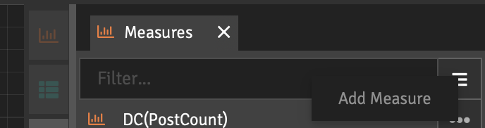
Based on columns from data tables, we can create measures. Measures are an aggregation of data in a column that includes the calculation of the number of records, sum of numbers in a column, maximum, minimum and average values, etc. Measures are created with the help of the Measures tab on the right menu. 

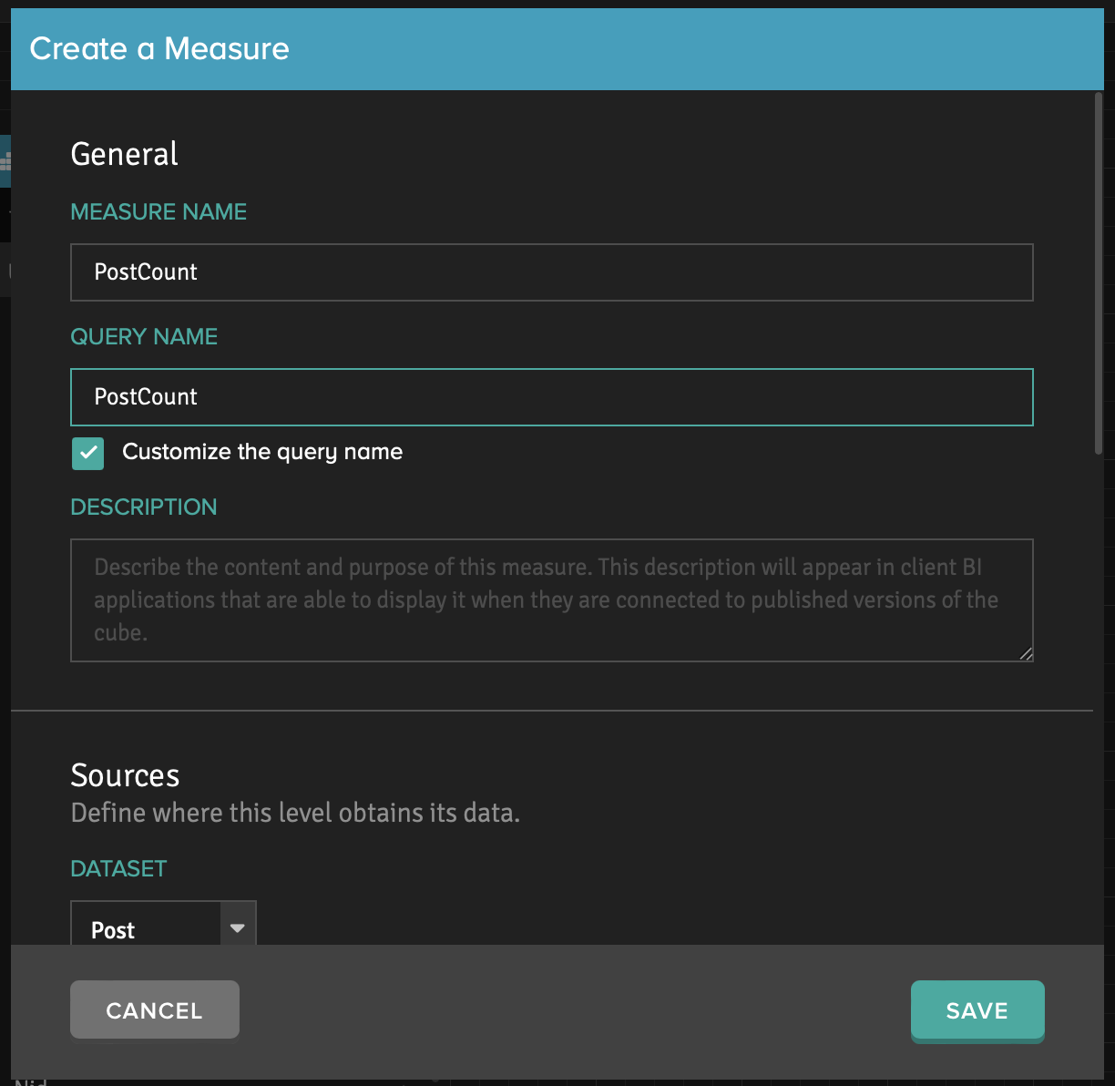
We should select from which table and which of its columns we will use the data to create the measure, as well as the aggregation function applied to those columns. Each measure has 2 names. The first one is displayed in the Adaptive Analytics interface. The second name is generated automatically by the column name and aggregation type and is indicated in the BI systems. We can change the second name of measure to our own choice, and it is a good idea to take this opportunity.

Using the same principle, we also can build dimensions with non-aggregated data from one column. Adaptive Analytics has two types of dimensions - actual and degenerate ones. Degenerate dimensions include all records from the columns bound to them, while not linking the tables to each other. Normal dimensions are based on one column of one table,  that is why they allow us to select only unique values from the column. However, other tables can be linked to this dimension too. When the data for records has no key in the dimension, it is simply ignored. For example, if the main table does not have a specific date, then data from related tables for this date will be skipped in calculations since there is no such member in the dimension.

From a usability point of view, degenerate dimensions are more convenient compared to actual ones. It happens because they make it impossible to lose data or establish unintended relationships between cubes in a project. However, from a performance point of view, the use of normal dimensions is preferable.

Dimensions are created in the corresponding tab on the right panel. We should specify the table and its column, from where we will get all unique values to fill the dimension. At the same time, we can use one column as a source of keys for the dimension, whereas the data from another one will fall into the actual dimension. For example, we can use the user's ID as a key, and moderately send his name. Therefore, users with the same name will be different entities for the measure.

Degenerate dimensions are created by dragging a column from a table from the workspace to the Dimensions tab. After that, the corresponding dimension is automatically assembled in the workspace.

All dimensions are organized in a hierarchical structure, even if there is only one of them. The structure has three levels. The first one is the name of the structure itself. The second one is the name of the hierarchy. The third level is the actual dimension in the hierarchy. A structure can have multiple hierarchies.

Using the created measures and dimensions, we can develop calculated measures. These are measures that were made with the help of the cut-off MDX language. They can do simple transformations with data in an OLAP structure, which is sometimes a practical feature.

Once you have assembled data structure, you can test it using a simple built-in previewer. To do this, go to the Cube Data Preview tab on the top menu of the workspace. Enter measures in Rows and dimensions in Columns or vice versa. This viewer is similar to Analysts in IRIS but with less functionality.

Knowing that our data structure works, we can set up our project to return data. To do this, click the “Publish” button on the main screen of the project. 

After that, the project immediately becomes available via the generated link. To get this link, we need to go to the published version of any of the cubes. To do that, open the cube in the Published section on the left menu. Go to the Connect tab and copy the link for the JDBC connection from the cube. It will be different for each project but the same for all the cubes in a project.

When you finish editing cubes and want to save changes, go to the export tab of the project and download the XML representation of your cube. Then put this file in the “/atscale-server/src/cubes/” folder of the repository (the file name doesn't matter) and delete the existing XML file of the project. If you don't delete the original file, Adaptive Analytics will not publish the updated project with the same name and ID. At the next build, a new version of the project will be automatically passed to Adaptive Analytics and will be ready for use as a default project.

We have figured out the basic functionality of Adaptive Analytics for now so let's talk about optimizing the execution time of analytical queries using UDAF. I will explain what benefits it gives us, and what problems might arise in this case.

UDAF stands for USER Defined aggregate functions. UDAF gives AtScale 2 main advantages. The first one is the ability to store query cash (they call it Aggregate Tables). It allows the next query to take already pre-calculated results from the database, using aggregation of data. The second one is the ability to use additional functions (actually User-Defined Aggregate Functions) and data processing algorithms that Adaptive Analytics is forced to store in the data source. They are kept in the database in a separate table, and Adaptive Analytics can call them by name in auto-generated queries. When Adaptive Analytics can use these functions, the performance of analytics queries increases dramatically.

The UDAF component must be installed in IRIS. It can be done manually (check the documentation about UDAF  on https://docs.intersystems.com/irisforhealthlatest/csp/docbook/DocBook.UI.Page.cls?KEY=AADAN#AADAN_config) or by installing a UDAF package from IPM (InterSystems Package Manager). At UDAF Adaptive Analytics Data Warehouse settings, change Custom Function Installation Mode to Custom Managed value.

The problem that appears when using aggregates is that such tables store outdated information at the time of the request. After the aggregate table is built, new values ​​that come to the data source are not added to aggregation tables. In order for aggregate tables to contain the freshest data possible, queries for them must be restarted, and new results should be written in the table.

Adaptive Analytics has an internal logic for updating aggregate tables, but it is much more convenient to control this process yourself. You can configure updates on a per-cube basis in the web interface of Adaptive Analytics and then use scripts from repository DC-analytics (https://github.com/teccod/Public-InterSystems-Developer-Community-analyt...) to export schedules and import them to another instance, or use the exported schedule file as a backup. You will also find a script to set all cubes to the same update schedule if you do not want to configure each one individually.

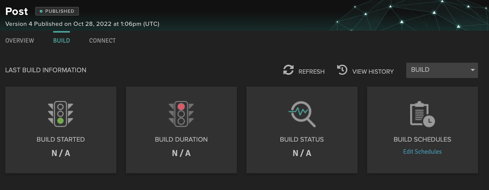
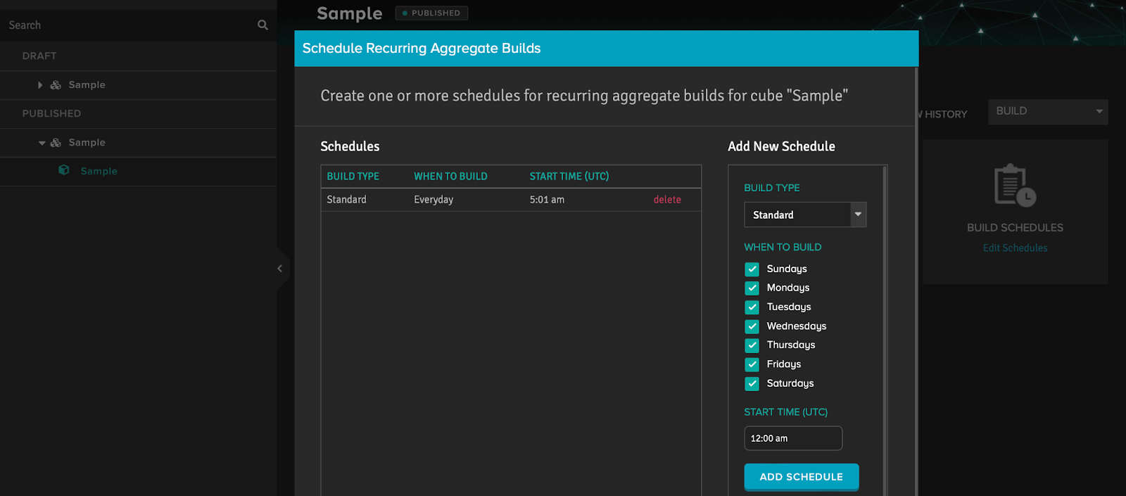
To set the schedule for updating aggregates in the Adaptive Analytics interface, we need to get into the published cube of the project (the procedure was described earlier). In the cube, go to the Build tab and find the window for managing the aggregation update schedule for this cube using the “Edin schedules” link. An easy-to-use editor will open up. Use it to set up a schedule for periodically updating data in the aggregate tables.

Thus, we have considered all main aspects of working with Adaptive Analytics. Of course, there are quite a lot of features and settings that we have not reviewed in this article. However, I am sure that if you need to use some of the options we haven't examined, it will not be difficult for you to figure things out on your own.